Example 5: Multi-state FBR-SOP tutorial (LVC model)
run type |
wavefunction |
backend |
Basis |
steps |
|---|---|---|---|---|
propagation |
MPS-SM |
Numpy |
HO-FBR |
200 |
Note
The use of PolynomialHamiltonian is deprecated. Use MPO style instead. See also other examples
1. Import modules
[1]:
from discvar import PrimBas_HO

from pytdscf import BasInfo, Model, Simulator, __version__
from pytdscf.hamiltonian_cls import PolynomialHamiltonian

__version__
[1]:
'1.2.0'
2. Define basis funciton
In this case, 2-state 3-mode simulation of N=10, ω1=1500 cm-1, ω2=2000 cm-1, ω3=2500 cm-1 are defined
[2]:
freqs_cm1 = [1500, 2000, 2500]
disps = [0.3, 0.4, 0.5]
nprim = 10
s0 = [PrimBas_HO(0.0, freq, nprim) for freq in freqs_cm1]
s1 = [
    PrimBas_HO(disp, freq, nprim)
    for freq, disp in zip(freqs_cm1, disps, strict=False)
]  # S1 basis is displaced from S0 basis
basinfo = BasInfo([s0, s1])
3. Define Hamiltonian
In this case, Hamiltonian is defined by
\[\begin{split}H=\left[\begin{array}{cc}
\sum_v-\frac{\omega_v}{2}\left(\frac{\partial^2}{\partial Q_v^2}+Q_v^2\right) & J_{12} + \sum_v \lambda_{12}^{(v)} Q_v\\
J_{21} + \sum_v \lambda_{21}^{(v)} Q_v& \sum_v-\frac{\omega_v}{2}\left(\frac{\partial^2}{\partial Q_v^2}+ (Q_v - Q^{(0)})^2\right)+\Delta E
\end{array}\right].\end{split}\]
[3]:
coupleJ = 0.0001  # J_12 and J_21 in a.u.
deltaE = 0.01  # ΔE in a.u.

hamiltonian = PolynomialHamiltonian(basinfo.get_ndof(), basinfo.get_nstate())
hamiltonian.coupleJ = [
    [-deltaE / 2, coupleJ],
    [coupleJ, deltaE / 2],
]  # Shifting diagonal term reduces the iteration of each step.

lam = {
    (0, 1): {0: 0.001, 1: 0.0001},
    (1, 0): {0: 0.001, 1: 0.0001},
}  # λ_12^(v) in Hartree / (sqrt(AMU) * Bohr)

hamiltonian.set_LVC(basinfo, lam)

operators = {"hamiltonian": hamiltonian}
4. Define misc
MPS bond-dimension is m=4
Initial population of 1-state is 1.0
Initial vibrational state is \(|0,0,0\rangle \otimes |1,0,0\rangle\) (only S0 state 0-th mode is excited)
[4]:
model = Model(basinfo, operators, bond_dim=4)
model.init_weight_ESTATE = [0.0, 1.0]
vib_gs = [1.0] + [0.0] * 9
vib_es = [0.0] + [1.0] + [0.0] * 8
model.init_weight_VIB_GS = [[vib_gs, vib_gs, vib_gs], [vib_es, vib_gs, vib_gs]]
# model.primbas_gs = list(itertools.chain.from_iterable([s0 for _ in range(nmol)]))
5. Execute simulation
Δt=0.1 fs
If
proj_gs=True, then the initial vibrational state is projected frommodel.primbas_gs.
[5]:
jobname = "LVC"
backend = "numpy"
simulator = Simulator(jobname, model, backend=backend, proj_gs=False)
simulator.propagate(maxstep=200, stepsize=0.1)
13:56:28 | INFO | Log file is ./LVC_prop/main.log
13:56:28 | WARNING | Employing sum of product Hamiltonian is deprecated.
13:56:28 | WARNING | Sum-of-Products (SOP) based calculation will be executed, but it is inefficient and will be deprecated, use Conventional MPO or Grid-MPO based calculation instead. See example such as https://qclovers.github.io/PyTDSCF/notebook/TD_reduced_density_exciton.html and https://kenhino.github.io/PyMPO/example/pytdscf-taylor.html
13:56:28 | INFO | Wave function is saved in wf_LVC.pkl
13:56:28 | INFO | Start initial step    0.000 [fs]
13:56:28 | INFO | End     0 step; propagated    0.100 [fs]; AVG Krylov iteration: 7.00
13:56:35 | INFO | End   100 step; propagated   10.100 [fs]; AVG Krylov iteration: 7.00
13:56:41 | INFO | End   199 step; propagated   19.900 [fs]; AVG Krylov iteration: 7.00
13:56:41 | INFO | End simulation and save wavefunction
13:56:41 | INFO | Wave function is saved in wf_LVC.pkl
[5]:
(0.01866900575908817, <pytdscf.wavefunction.WFunc at 0x7f16a40e4050>)
[6]:
!cat LVC_prop/populations.dat
# time [fs]     pop_0           pop_1
0.000000000     0.000000000     1.000000000
0.100000000     0.001514000     0.998486000
0.200000000     0.006028346     0.993971654
0.300000000     0.013461024     0.986538976
0.400000000     0.023678470     0.976321530
0.500000000     0.036500074     0.963499926
0.600000000     0.051704140     0.948295860
0.700000000     0.069034987     0.930965013
0.800000000     0.088210837     0.911789163
0.900000000     0.108932106     0.891067894
1.000000000     0.130889748     0.869110252
1.100000000     0.153773302     0.846226698
1.200000000     0.177278383     0.822721617
1.300000000     0.201113394     0.798886606
1.400000000     0.225005317     0.774994683
1.500000000     0.248704516     0.751295484
1.600000000     0.271988515     0.728011485
1.700000000     0.294664789     0.705335211
1.800000000     0.316572583     0.683427417
1.900000000     0.337583842     0.662416158
2.000000000     0.357603259     0.642396741
2.100000000     0.376567512     0.623432488
2.200000000     0.394443690     0.605556310
2.300000000     0.411226947     0.588773053
2.400000000     0.426937427     0.573062573
2.500000000     0.441616516     0.558383484
2.600000000     0.455322550     0.544677450
2.700000000     0.468126111     0.531873889
2.800000000     0.480105146     0.519894854
2.900000000     0.491340139     0.508659861
3.000000000     0.501909607     0.498090393
3.100000000     0.511886182     0.488113818
3.200000000     0.521333495     0.478666505
3.300000000     0.530304015     0.469695985
3.400000000     0.538837908     0.461162092
3.500000000     0.546962858     0.453037142
3.600000000     0.554694719     0.445305281
3.700000000     0.562038759     0.437961241
3.800000000     0.568991208     0.431008792
3.900000000     0.575540834     0.424459166
4.000000000     0.581670269     0.418329731
4.100000000     0.587356927     0.412643073
4.200000000     0.592573419     0.407426581
4.300000000     0.597287542     0.402712458
4.400000000     0.601461995     0.398538005
4.500000000     0.605054079     0.394945921
4.600000000     0.608015702     0.391984298
4.700000000     0.610293975     0.389706025
4.800000000     0.611832638     0.388167362
4.900000000     0.612574441     0.387425559
5.000000000     0.612464453     0.387535547
5.100000000     0.611454125     0.388545875
5.200000000     0.609505782     0.390494218
5.300000000     0.606597131     0.393402869
5.400000000     0.602725305     0.397274695
5.500000000     0.597910013     0.402089987
5.600000000     0.592195416     0.407804584
5.700000000     0.585650526     0.414349474
5.800000000     0.578368064     0.421631936
5.900000000     0.570461906     0.429538094
6.000000000     0.562063393     0.437936607
6.100000000     0.553316883     0.446683117
6.200000000     0.544374973     0.455625027
6.300000000     0.535393777     0.464606223
6.400000000     0.526528586     0.473471414
6.500000000     0.517930062     0.482069938
6.600000000     0.509741033     0.490258967
6.700000000     0.502093758     0.497906242
6.800000000     0.495107498     0.504892502
6.900000000     0.488886159     0.511113841
7.000000000     0.483515836     0.516484164
7.100000000     0.479062191     0.520937809
7.200000000     0.475567725     0.524432275
7.300000000     0.473049199     0.526950801
7.400000000     0.471495580     0.528504420
7.500000000     0.470866997     0.529133003
7.600000000     0.471095168     0.528904832
7.700000000     0.472085710     0.527914290
7.800000000     0.473722501     0.526277499
7.900000000     0.475874069     0.524125931
8.000000000     0.478401609     0.521598391
8.100000000     0.481167989     0.518832011
8.200000000     0.484046854     0.515953146
8.300000000     0.486930803     0.513069197
8.400000000     0.489737646     0.510262354
8.500000000     0.492413894     0.507586106
8.600000000     0.494934969     0.505065031
8.700000000     0.497301996     0.502698004
8.800000000     0.499535556     0.500464444
8.900000000     0.501667184     0.498332816
9.000000000     0.503729776     0.496270224
9.100000000     0.505748293     0.494251707
9.200000000     0.507732148     0.492267852
9.300000000     0.509670500     0.490329500
9.400000000     0.511531305     0.488468695
9.500000000     0.513264444     0.486735556
9.600000000     0.514808668     0.485191332
9.700000000     0.516101518     0.483898482
9.800000000     0.517090879     0.482909121
9.900000000     0.517746516     0.482253484
10.000000000    0.518069862     0.481930138
10.100000000    0.518100437     0.481899563
10.200000000    0.517917722     0.482082278
10.300000000    0.517637835     0.482362165
10.400000000    0.517405063     0.482594937
10.500000000    0.517379013     0.482620987
10.600000000    0.517718752     0.482281248
10.700000000    0.518565763     0.481434237
10.800000000    0.520027787     0.479972213
10.900000000    0.522165532     0.477834468
11.000000000    0.524983940     0.475016060
11.100000000    0.528429158     0.471570842
11.200000000    0.532391652     0.467608348
11.300000000    0.536715158     0.463284842
11.400000000    0.541210448     0.458789552
11.500000000    0.545672319     0.454327681
11.600000000    0.549897849     0.450102151
11.700000000    0.553703868     0.446296132
11.800000000    0.556941747     0.443058253
11.900000000    0.559508005     0.440491995
12.000000000    0.561349828     0.438650172
12.100000000    0.562465233     0.437534767
12.200000000    0.562898300     0.437101700
12.300000000    0.562730479     0.437269521
12.400000000    0.562069371     0.437930629
12.500000000    0.561036619     0.438963381
12.600000000    0.559756521     0.440243479
12.700000000    0.558346714     0.441653286
12.800000000    0.556911932     0.443088068
12.900000000    0.555541280     0.444458720
13.000000000    0.554308964     0.445691036
13.100000000    0.553277910     0.446722090
13.200000000    0.552505331     0.447494669
13.300000000    0.552049054     0.447950946
13.400000000    0.551973391     0.448026609
13.500000000    0.552353429     0.447646571
13.600000000    0.553276901     0.446723099
13.700000000    0.554843148     0.445156852
13.800000000    0.557159088     0.442840912
13.900000000    0.560332544     0.439667456
14.000000000    0.564463569     0.435536431
14.100000000    0.569634697     0.430365303
14.200000000    0.575901146     0.424098854
14.300000000    0.583282004     0.416717996
14.400000000    0.591753310     0.408246690
14.500000000    0.601243730     0.398756270
14.600000000    0.611633273     0.388366727
14.700000000    0.622755188     0.377244812
14.800000000    0.634400901     0.365599099
14.900000000    0.646327607     0.353672393
15.000000000    0.658267936     0.341732064
15.100000000    0.669940970     0.330059030
15.200000000    0.681063838     0.318936162
15.300000000    0.691363131     0.308636869
15.400000000    0.700585399     0.299414601
15.500000000    0.708506152     0.291493848
15.600000000    0.714936901     0.285063099
15.700000000    0.719729945     0.280270055
15.800000000    0.722780782     0.277219218
15.900000000    0.724028234     0.275971766
16.000000000    0.723452480     0.276547520
16.100000000    0.721071376     0.278928624
16.200000000    0.716935545     0.283064455
16.300000000    0.711122734     0.288877266
16.400000000    0.703732025     0.296267975
16.500000000    0.694878366     0.305121634
16.600000000    0.684687868     0.315312132
16.700000000    0.673294116     0.326705884
16.800000000    0.660835644     0.339164356
16.900000000    0.647454495     0.352545505
17.000000000    0.633295651     0.366704349
17.100000000    0.618507001     0.381492999
17.200000000    0.603239403     0.396760597
17.300000000    0.587646403     0.412353597
17.400000000    0.571883224     0.428116776
17.500000000    0.556104733     0.443895267
17.600000000    0.540462285     0.459537715
17.700000000    0.525099509     0.474900491
17.800000000    0.510147305     0.489852695
17.900000000    0.495718504     0.504281496
18.000000000    0.481902722     0.518097278
18.100000000    0.468762025     0.531237975
18.200000000    0.456327965     0.543672035
18.300000000    0.444600424     0.555399576
18.400000000    0.433548562     0.566451438
18.500000000    0.423113890     0.576886110
18.600000000    0.413215304     0.586784696
18.700000000    0.403755665     0.596244335
18.800000000    0.394629355     0.605370645
18.900000000    0.385730116     0.614269884
19.000000000    0.376958495     0.623041505
19.100000000    0.368228232     0.631771768
19.200000000    0.359471110     0.640528890
19.300000000    0.350639950     0.649360050
19.400000000    0.341709672     0.658290328
19.500000000    0.332676566     0.667323434
19.600000000    0.323556112     0.676443888
19.700000000    0.314379815     0.685620185
19.800000000    0.305191620     0.694808380
19.900000000    0.296044446     0.703955554
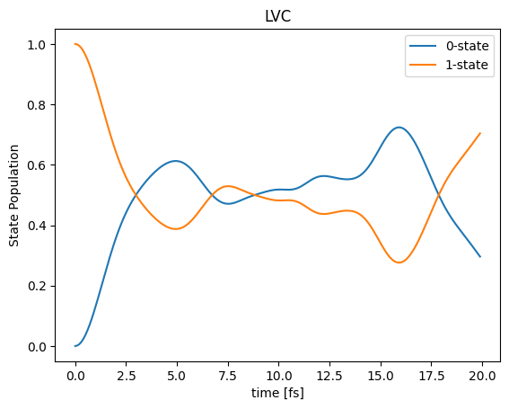
7. Visualize populations
[7]:
# !gnuplot -e " set xlabel 'time [fs]'; set ylabel 'population'; plot 'PropagateMultiStateSOP/populations.log' using 1:2 with lines title '0-state', 'PropagateMultiStateSOP/populations.log' using 1:3 with lines title '1-state'"
import matplotlib.pyplot as plt
import numpy as np

data = np.loadtxt("LVC_prop/populations.dat")

plt.plot(data[:, 0], data[:, 1], label="0-state")
plt.plot(data[:, 0], data[:, 2], label="1-state")

plt.title(jobname)
plt.xlabel("time [fs]")
plt.ylabel("State Population")

plt.legend()
plt.show()
[ ]: