Example 14 Electron and nuclear spin mixed state dynamics with RadicalPy
In this tutorial, one constructs MPO of radical pair system (two electron spins and a couple of nuclear spins under magnetic field) by using RadicalPy library.
Import required modules
[1]:
try:
    import radicalpy
except ModuleNotFoundError:
    # remove uv if you are not using uv
    !uv pip install radicalpy --quiet

!uv pip show radicalpy

import pytdscf

pytdscf.__version__
Using Python 3.12.2 environment at /Users/hinom/GitHub/PyTDSCF/.venv
Name: radicalpy
Version: 1.0.9
Location: /Users/hinom/GitHub/PyTDSCF/.venv/lib/python3.12/site-packages
Requires: dot2tex, graphviz, importlib-resources, matplotlib, mdanalysis, numpy, pint, rdkit, scikit-learn, scipy, seaborn, sympy, tqdm
Required-by:
[1]:
'1.3.1'
[2]:
from math import isqrt

import matplotlib.pyplot as plt
import numpy as np
import radicalpy as rp
from IPython.display import HTML
from pympo import (
    AssignManager,
    OpSite,
    SumOfProducts,
)
from radicalpy.simulation import State
from sympy import Symbol

from pytdscf import Exciton, Model, Simulator, units
from pytdscf.util import get_anim, read_nc
Vectorisation of density matrix
Density matrix \(\rho \in \mathbb{C}^{d \times d}\) can be “vectorised” as
where
Thus, one-dimensional index (in the sense of column-major order, density matrix: ket->bra) is defined as
and
If one adopt basis \(\{|i\rangle\}\),
Now, dual operation \(A\rho B^\dagger\) can be vectorised as
Proof >
>
Vectorisation of the von Neumann equation
von Neumann equation is
Thus, its vectorised form is
Note
Since the density matrix is approximated by MPS, there are no guarantee that \(\rho = \rho^\dagger\) (Hermitian), \(\rho_{ii} \geq 0\) (positive semi-definite) and \(\mathrm{Tr}(\rho) = 1\) (normalized).
Total Hamiltonian
Define systems
[3]:
is_small_case = True

if is_small_case:
    # You can use following block instead
    n_nuc_spins = 1

    flavin = rp.simulation.Molecule.fromisotopes(
        isotopes=["1H"] * n_nuc_spins, hfcs=[0.4] * n_nuc_spins
    )
    Z = rp.simulation.Molecule.fromisotopes(
        isotopes=["14N"] * n_nuc_spins, hfcs=[0.5] * n_nuc_spins
    )
    sim = rp.simulation.LiouvilleSimulation([flavin, Z])

    # Parameters
    A = {}  # mT
    isotropic = True

    # Isotropic
    for i in range(len(sim.radicals)):
        for j, nuc in enumerate(sim.molecules[i].nuclei):
            if isotropic:
                A[(i, j)] = np.eye(3) * nuc.hfc.isotropic
            else:
                A[(i, j)] = nuc.hfc.anisotropic
    B0 = 0.2  # 2J
    B = np.array((0.0, 0.0, 1.0)) * B0  # mT
    J = 0.1  # Typically 1.0e+03 scale # mT
    D = -0.1  # mT
    kS = 1.0e06  # Exponential model in s-1
    kT = 1.0e06
    if isinstance(D, float):
        assert D <= 0
        D = 2 / 3 * np.diag((-1.0, -1.0, 2.0)) * D
else:
    flavin = rp.simulation.Molecule.all_nuclei("flavin_anion")
    trp = rp.simulation.Molecule.all_nuclei("tryptophan_cation")
    sim = rp.simulation.LiouvilleSimulation([flavin, trp])
    A = {}
    isotropic = False
    for i in range(len(sim.radicals)):
        for j, nuc in enumerate(sim.molecules[i].nuclei):
            if isotropic:
                A[(i, j)] = np.eye(3) * nuc.hfc.isotropic
            else:
                A[(i, j)] = nuc.hfc.anisotropic
    B0 = 2.0  # Typically 0.01 mT~10 mT
    B = np.array((0.0, 0.0, 1.0)) * B0
    J = 0.1  # Typically 1.0e+03 scale
    D = -0.1
    kS = 1.0e06  # Exponential model in s-1
    kT = 1.0e06
    if isinstance(D, float):
        assert D <= 0
        D = 2 / 3 * np.diag((-1.0, -1.0, 2.0)) * D
sim
[3]:
Number of electrons: 2
Number of nuclei: 2
Number of particles: 4
Multiplicities: [2, 2, 2, 3]
Magnetogyric ratios (mT): [-176085963.023, -176085963.023, 267522.18744, 19337.792]
Nuclei: [1H(267522187.44, 2, 0.4 <anisotropic not available>), 14N(19337792.0, 3, 0.5 <anisotropic not available>)]
Couplings: [0, 1]
HFCs (mT): [0.4 <anisotropic not available>, 0.5 <anisotropic not available>]
Now, one defines matrix product state (MPS) in the following order
(nuclei in flavin) \(\to\) (electronic states \(\{|T_{+}\rangle, |T_{0}\rangle, |S\rangle, |T_{-}\rangle\}\)) \(\to\) (neclei in Z)
Extract one particle operator
RadicalPy provides variety of spin operators such as
\(\hat{s}_x, \hat{s}_y, \hat{s}_z\) for radical singlet-triplet basis
\(\hat{I}_x, \hat{I}_y, \hat{I}_z\) for nuclear Zeeman basis
[4]:
# Clear nuclei temporally
_nuclei_tmp0 = sim.molecules[0].nuclei
_nuclei_tmp1 = sim.molecules[1].nuclei
sim.molecules[0].nuclei = []
sim.molecules[1].nuclei = []
# for Singlet-Triplet basis
sx_1 = sim.spin_operator(0, "x")
sy_1 = sim.spin_operator(0, "y")
sz_1 = sim.spin_operator(0, "z")
sx_2 = sim.spin_operator(1, "x")
sy_2 = sim.spin_operator(1, "y")
sz_2 = sim.spin_operator(1, "z")
Qs = sim.projection_operator(rp.simulation.State.SINGLET)
Qt = sim.projection_operator(rp.simulation.State.TRIPLET)
# Revert nuclei
sim.molecules[0].nuclei = _nuclei_tmp0
sim.molecules[1].nuclei = _nuclei_tmp1
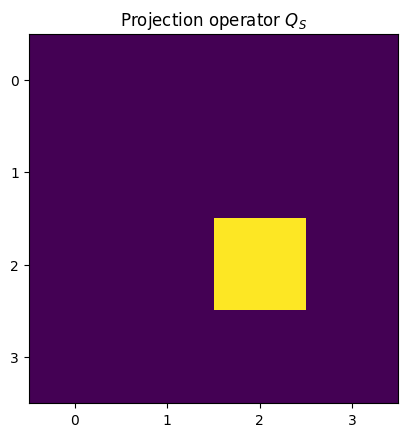
plt.title("Projection operator $Q_S$")
plt.imshow(Qs.real)
plt.xticks([0, 1, 2, 3])
plt.yticks([0, 1, 2, 3])
plt.show()
Define OpSite and coefficients
RadicalPy uses Hz in energy unit but it is too large to keep numerical stabiltiy
Thus, one will use GHz in energy unit
For some reasons, extraction of imaginary unit of pauli y operator leads stable simulation for degenerate system (why??)
[5]:
SCALE = 1.0e-09
gamma = [p.gamma_mT for p in sim.particles]

g_ele_sym = [
    Symbol(r"\gamma_e^{(" + f"{i + 1}" + ")}") for i in range(len(sim.radicals))
]
g_nuc_sym = {}
for i in range(len(sim.radicals)):
    for j in range(len(sim.molecules[i].nuclei)):
        g_nuc_sym[(i, j)] = Symbol(r"\gamma_n^{" + f"{(i + 1, j + 1)}" + "}")

subs = {}
for i, ge in enumerate(g_ele_sym):
    subs[ge] = sim.radicals[i].gamma_mT
for (i, j), gn in g_nuc_sym.items():
    subs[gn] = sim.molecules[i].nuclei[j].gamma_mT
Define radical spin operators
[6]:
def get_OE(op):
    """
    OT ⊗ 𝟙
    """
    return np.kron(op.T, np.eye(op.shape[0], dtype=op.dtype))


def get_EO(op):
    """
    𝟙 ⊗ O
    """
    return np.kron(np.eye(op.shape[0], dtype=op.dtype), op)


ele_site = len(sim.molecules[0].nuclei)

SxE_ops = []
SyE_ops = []
SzE_ops = []
ESx_ops = []
ESy_ops = []
ESz_ops = []

S1S2E_op = OpSite(
    r"(\hat{S}_1\cdot\hat{S}_2)^\ast ⊗ 𝟙",
    ele_site,
    value=get_OE(sx_1 @ sx_2 + sy_1 @ sy_2 + sz_1 @ sz_2),
)
ES1S2_op = OpSite(
    r"𝟙 ⊗ (\hat{S}_1\cdot\hat{S}_2)",
    ele_site,
    value=get_EO(sx_1 @ sx_2 + sy_1 @ sy_2 + sz_1 @ sz_2),
)
EE_op = OpSite(
    r"\hat{E} ⊗ \hat{E}", ele_site, value=get_OE(np.eye(sx_1.shape[0]))
)

QsE_op = OpSite(r"\hat{Q}_S ⊗ 𝟙", ele_site, value=get_OE(Qs))
EQs_op = OpSite(r"𝟙 ⊗ \hat{Q}_S", ele_site, value=get_EO(Qs))
QtE_op = OpSite(r"\hat{Q}_T ⊗ 𝟙", ele_site, value=get_OE(Qt))
EQt_op = OpSite(r"𝟙 ⊗ \hat{Q}_T", ele_site, value=get_EO(Qt))


SxE_ops.append(OpSite(r"\hat{S}_x^{(1)\ast} ⊗ 𝟙", ele_site, value=get_OE(sx_1)))
SxE_ops.append(OpSite(r"\hat{S}_x^{(2)\ast} ⊗ 𝟙", ele_site, value=get_OE(sx_2)))
SyE_ops.append(OpSite(r"\hat{S}_y^{(1)\ast} ⊗ 𝟙", ele_site, value=get_OE(sy_1)))
SyE_ops.append(OpSite(r"\hat{S}_y^{(2)\ast} ⊗ 𝟙", ele_site, value=get_OE(sy_2)))
SzE_ops.append(OpSite(r"\hat{S}_z^{(1)\ast} ⊗ 𝟙", ele_site, value=get_OE(sz_1)))
SzE_ops.append(OpSite(r"\hat{S}_z^{(2)\ast} ⊗ 𝟙", ele_site, value=get_OE(sz_2)))

ESx_ops.append(OpSite(r"𝟙 ⊗ \hat{S}_x^{(1)}", ele_site, value=get_EO(sx_1)))
ESx_ops.append(OpSite(r"𝟙 ⊗ \hat{S}_x^{(2)}", ele_site, value=get_EO(sx_2)))
ESy_ops.append(OpSite(r"𝟙 ⊗ \hat{S}_y^{(1)}", ele_site, value=get_EO(sy_1)))
ESy_ops.append(OpSite(r"𝟙 ⊗ \hat{S}_y^{(2)}", ele_site, value=get_EO(sy_2)))
ESz_ops.append(OpSite(r"𝟙 ⊗ \hat{S}_z^{(1)}", ele_site, value=get_EO(sz_1)))
ESz_ops.append(OpSite(r"𝟙 ⊗ \hat{S}_z^{(2)}", ele_site, value=get_EO(sz_2)))

SrE_ops = [SxE_ops, SyE_ops, SzE_ops]
ESr_ops = [ESx_ops, ESy_ops, ESz_ops]
Define nuclear spin operators
[7]:
IxE_ops = {}
IyE_ops = {}
IzE_ops = {}
EIx_ops = {}
EIy_ops = {}
EIz_ops = {}

for j, nuc in enumerate(sim.molecules[0].nuclei):
    val = nuc.pauli["x"]
    IxE_ops[(0, j)] = OpSite(
        r"\hat{I}_x^{" + f"{(1, j + 1)}" + r"\ast} ⊗ 𝟙",
        j,
        value=get_OE(val),
    )
    EIx_ops[(0, j)] = OpSite(
        r"𝟙 ⊗ \hat{I}_x^{" + f"{(1, j + 1)}" + "}",
        j,
        value=get_EO(val),
    )
    val = nuc.pauli["y"]
    IyE_ops[(0, j)] = OpSite(
        r"\hat{I}_y^{" + f"{(1, j + 1)}" + r"\ast} ⊗ 𝟙",
        j,
        value=get_OE(val),
    )
    EIy_ops[(0, j)] = OpSite(
        r"𝟙 ⊗ \hat{I}_y^{" + f"{(1, j + 1)}" + "}",
        j,
        value=get_EO(val),
    )
    val = nuc.pauli["z"]
    IzE_ops[(0, j)] = OpSite(
        r"\hat{I}_z^{" + f"{(1, j + 1)}" + r"\ast} ⊗ 𝟙",
        j,
        value=get_OE(val),
    )
    EIz_ops[(0, j)] = OpSite(
        r"𝟙 ⊗ \hat{I}_z^{" + f"{(1, j + 1)}" + "}",
        j,
        value=get_EO(val),
    )

for j, nuc in enumerate(sim.molecules[1].nuclei):
    site = ele_site + 1 + j
    val = nuc.pauli["x"]
    IxE_ops[(1, j)] = OpSite(
        r"\hat{I}_x^{" + f"{(2, j + 1)}" + r"\ast} ⊗ 𝟙",
        site,
        value=get_OE(val),
    )
    EIx_ops[(1, j)] = OpSite(
        r"𝟙 ⊗ \hat{I}_x^{" + f"{(2, j + 1)}" + "}",
        site,
        value=get_EO(val),
    )
    val = nuc.pauli["y"]
    IyE_ops[(1, j)] = OpSite(
        r"\hat{I}_y^{" + f"{(2, j + 1)}" + r"\ast} ⊗ 𝟙",
        site,
        value=get_OE(val),
    )
    EIy_ops[(1, j)] = OpSite(
        r"𝟙 ⊗ \hat{I}_y^{" + f"{(2, j + 1)}" + "}",
        ele_site + 1 + j,
        value=get_EO(val),
    )
    val = nuc.pauli["z"]
    IzE_ops[(1, j)] = OpSite(
        r"\hat{I}_z^{" + f"{(2, j + 1)}" + r"\ast} ⊗ 𝟙",
        site,
        value=get_OE(val),
    )
    EIz_ops[(1, j)] = OpSite(
        r"𝟙 ⊗ \hat{I}_z^{" + f"{(2, j + 1)}" + "}",
        site,
        value=get_EO(val),
    )

IrE_ops = [IxE_ops, IyE_ops, IzE_ops]
EIr_ops = [EIx_ops, EIy_ops, EIz_ops]
Hyperfine coupling Hamiltonian
[8]:
hyperfine = SumOfProducts()

xyz = "xyz"

for i in range(len(sim.radicals)):
    for j in range(len(sim.molecules[i].nuclei)):
        for k, (SrE_op, ESr_op) in enumerate(
            zip(SrE_ops, ESr_ops, strict=True)
        ):
            for l, (IrE_op, EIr_op) in enumerate(
                zip(IrE_ops, EIr_ops, strict=True)
            ):
                if A[(i, j)][k, l] == 0.0:
                    continue
                Asym = Symbol(
                    "A^{"
                    + f"{(i + 1, j + 1)}"
                    + "}_{"
                    + f"{xyz[k]}"
                    + f"{xyz[l]}"
                    + "}"
                )
                subs[Asym] = A[(i, j)][k, l].item() * SCALE
                hyperfine -= (
                    Asym * abs(g_ele_sym[0]) * SrE_op[i] * IrE_op[(i, j)]
                )
                hyperfine += (
                    Asym * abs(g_ele_sym[0]) * ESr_op[i] * EIr_op[(i, j)]
                )
[9]:
hyperfine = hyperfine.simplify()
hyperfine.symbol
[9]:
Zeeman Hamiltonian
[10]:
zeeman = SumOfProducts()

xyz = "xyz"

for k, (SrE_op, ESr_op, IrE_op, EIr_op) in enumerate(
    zip(SrE_ops, ESr_ops, IrE_ops, EIr_ops, strict=True)
):
    if B[k] == 0.0:
        continue
    r = xyz[k]
    Br = Symbol(f"B_{r}")
    subs[Br] = B[k] * SCALE
    for i in range(len(sim.radicals)):
        zeeman += -Br * g_ele_sym[i] * ESr_op[i]
        zeeman += Br * g_ele_sym[i] * SrE_op[i]
        for j in range(len(sim.molecules[i].nuclei)):
            zeeman += -Br * g_nuc_sym[(i, j)] * EIr_op[(i, j)]
            zeeman += Br * g_nuc_sym[(i, j)] * IrE_op[(i, j)]

zeeman = zeeman.simplify()
zeeman.symbol
[10]:
Exchange Hamiltonian
[11]:
exchange = SumOfProducts()
if J != 0.0:
    Jsym = Symbol("J")
    subs[Jsym] = J * SCALE
    exchange += -Jsym * abs(g_ele_sym[0]) * (2 * ES1S2_op + 0.5 * EE_op)
    exchange -= -Jsym * abs(g_ele_sym[0]) * (2 * S1S2E_op + 0.5 * EE_op)
    exchange = exchange.simplify()
exchange.symbol
[11]:
Dipolar Hamiltonian
[12]:
dipolar = SumOfProducts()
for k in range(3):
    for l in range(3):
        if D[k, l] == 0.0:
            continue
        else:
            Dsym = Symbol("D_{" + f"{xyz[k]}" + f"{xyz[l]}" + "}")
            subs[Dsym] = D[k, l] * SCALE
            dipolar += Dsym * abs(g_ele_sym[0]) * ESr_ops[k][0] * ESr_ops[l][1]
            dipolar -= Dsym * abs(g_ele_sym[0]) * SrE_ops[k][0] * SrE_ops[l][1]
dipolar = dipolar.simplify()
dipolar.symbol
[12]:
Haberkorn relaxation
The superoperator for vectorised form density matrix is
[13]:
haberkorn = SumOfProducts()
if kS != 0.0:
    kSsym = Symbol("k_S")
    subs[kSsym] = kS * SCALE
    haberkorn -= 1.0j * kSsym / 2 * (QsE_op + EQs_op)
if kT != 0.0:
    kTsym = Symbol("k_T")
    subs[kTsym] = kT * SCALE
    haberkorn -= 1.0j * kTsym / 2 * (QtE_op + EQt_op)
haberkorn = haberkorn.simplify()
haberkorn.symbol
[13]:
Construct matrix product operator (MPO) for MPS propagation
[14]:
L = hyperfine + zeeman + exchange + dipolar + haberkorn
L = L.simplify()
am = AssignManager(L)
_ = am.assign()
# display(*am.Wsym)
mpo = am.numerical_mpo(subs=subs)
L.symbol
[14]:
Liouville simulation
[15]:
backend = "numpy"  # or "jax"  for large bond dimension and GPU
m = 32  # Bond dimension
Δt = 5.0e-10 / SCALE * units.au_in_fs  # dt = 0.5 ns
[16]:
basis = []
for nuc in sim.molecules[0].nuclei:
    basis.append(Exciton(nstate=nuc.multiplicity**2))
basis.append(Exciton(nstate=4**2))
for nuc in sim.molecules[1].nuclei:
    basis.append(Exciton(nstate=nuc.multiplicity**2))
nsite = len(basis)
[17]:
def singlet_state():
    hp = []
    for isite in range(nsite):
        if isite == ele_site:
            op = Qs
        else:
            # Mixed states !
            op = np.eye(isqrt(basis[isite].nstate))
        # Automatically nomarized so that trace=1 in internal code
        hp.append(op.reshape(-1).tolist())
    return hp


def process(mpo):
    operators = {"hamiltonian": mpo}
    model = Model(basis, operators=operators, space="Liouville", bond_dim=m)
    hp = singlet_state()
    model.init_HartreeProduct = [hp]

    jobname = "radicalpair_liouville"
    simulator = Simulator(
        jobname=jobname,
        model=model,
        backend=backend,
        verbose=0,
    )
    # Initiate the propagation setting with maxstep=0
    nstep = 100
    ener, wf = simulator.propagate(
        reduced_density=(
            [(ele_site, ele_site)],
            2,
        ),
        maxstep=nstep + 1,
        stepsize=Δt,
        autocorr=False,
        energy=False,
        norm=False,
        populations=False,
        observables=True,
        integrator="arnoldi",  # Since non-Hermitian
    )
    data = read_nc(f"{jobname}_prop/reduced_density.nc", [(ele_site, ele_site)])
    time_data = data["time"]
    density_data = data[(ele_site, ele_site)]
    return density_data, time_data
Since nuclear spins are mixed state, one needs to consider ensemble of nuclear spin initial states.
[18]:
dm, time_data = process(mpo)
time_data_μs = time_data * SCALE * 1e06 / units.au_in_fs
15:36:14 | INFO | Wave function is saved in wf_radicalpair_liouville.pkl
15:36:14 | INFO | The time unit in the netCDF file is fs
15:36:14 | INFO | Start initial step    0.000 [fs]
15:36:14 | INFO | End     0 step; propagated    0.012 [fs]; AVG Krylov iteration: 5.67
15:36:15 | INFO | End   100 step; propagated    1.209 [fs]; AVG Krylov iteration: 5.67
15:36:15 | INFO | End simulation and save wavefunction
15:36:15 | INFO | Wave function is saved in wf_radicalpair_liouville.pkl
[19]:
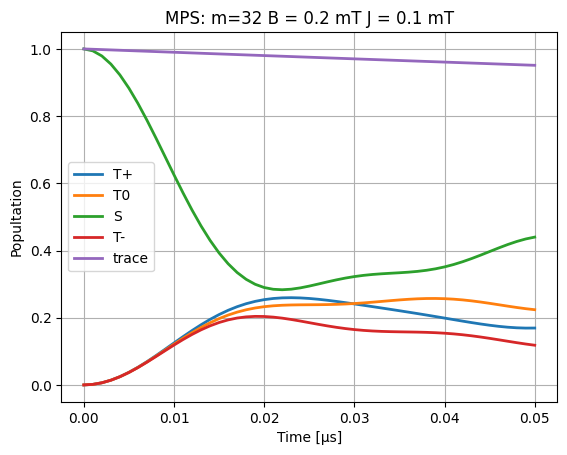
plt.plot(time_data_μs, dm[:, 0, 0].real, linewidth=2, label="T+")
plt.plot(time_data_μs, dm[:, 1, 1].real, linewidth=2, label="T0")
plt.plot(time_data_μs, dm[:, 2, 2].real, linewidth=2, label="S")
plt.plot(time_data_μs, dm[:, 3, 3].real, linewidth=2, label="T-")
plt.plot(time_data_μs, np.einsum("ijj->i", dm.real), linewidth=2, label="trace")
plt.title(f"MPS: {m=} B = {B0} mT J = {J} mT")
plt.legend()
plt.xlabel("Time [μs]")
plt.ylabel("Popultation")
plt.grid()
# plt.ylim([0, 1])
plt.savefig("population.png")
plt.show()
[20]:
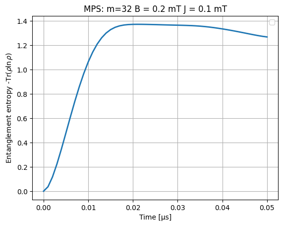
from scipy.linalg import logm

plt.plot(
    time_data_μs,
    [-np.trace(rho * logm(rho)).real for rho in dm],
    linewidth=2,
    label="",
)

plt.title(f"MPS: {m=} B = {B0} mT J = {J} mT")
plt.legend()
plt.xlabel("Time [μs]")
plt.ylabel(r"Entanglement entropy -Tr($\rho \ln \rho$)")
plt.grid()
plt.show()
/Users/hinom/GitHub/PyTDSCF/.venv/lib/python3.12/site-packages/scipy/linalg/_matfuncs.py:202: LogmExactlySingularWarning: The logm input matrix is exactly singular.
  F = scipy.linalg._matfuncs_inv_ssq._logm(A)
/var/folders/sj/nm7r7k8969b31b686cw52trh0000gn/T/ipykernel_29482/1577440271.py:11: UserWarning: No artists with labels found to put in legend.  Note that artists whose label start with an underscore are ignored when legend() is called with no argument.
  plt.legend()
[21]:
# Note: spin coherent state sampling has slower convergence for off-diagnal term than projection state sampling
fig, anim = get_anim(
    dm[::2, :, :],
    time_data_μs[::2],
    title="Reduced density matrix",
    time_unit="μs",
    save_gif=True,
    dpi=30,
    gif_filename="rdm-radical.gif",
    row_names=[
        r"$|T+\rangle$",
        r"$|T0\rangle$",
        r"$|S\rangle$",
        r"$|T-\rangle$",
    ],
    col_names=[
        r"$\langle T+|$",
        r"$\langle T0|$",
        r"$\langle S|$",
        r"$\langle T-|$",
    ],
)
plt.show()
HTML(anim.to_jshtml())
Saving animation to rdm-radical.gif...
Animation saved successfully!
[21]:
Compare with RadicalPy simulation
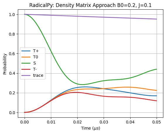
[22]:
if len(basis) < 6:
    assert isinstance(D, np.ndarray)
    H = sim.total_hamiltonian(B0=B0, D=D, J=J)
    time = np.arange(0, 5.0e-8 + 5e-10, 5e-10)
    kinetics = [
        rp.kinetics.Haberkorn(kS, rp.simulation.State.SINGLET),
        rp.kinetics.Haberkorn(kT, rp.simulation.State.TRIPLET),
    ]
    sim.apply_liouville_hamiltonian_modifiers(H, kinetics)
    rhos = sim.time_evolution(State.SINGLET, time, H)

    time_evol_s = sim.product_probability(State.SINGLET, rhos)
    time_evol_tp = sim.product_probability(State.TRIPLET_PLUS, rhos)
    time_evol_tz = sim.product_probability(State.TRIPLET_ZERO, rhos)
    time_evol_tm = sim.product_probability(State.TRIPLET_MINUS, rhos)
    x = time * 1e6

    plt.plot(x, time_evol_tp, linewidth=2, label="T+")
    plt.plot(x, time_evol_tz, linewidth=2, label="T0")
    plt.plot(x, time_evol_s, linewidth=2, label="S")
    plt.plot(x, time_evol_tm, linewidth=2, label="T-")
    plt.plot(
        x,
        time_evol_tp + time_evol_tz + time_evol_s + time_evol_tm,
        linewidth=2,
        label="trace",
    )
    plt.legend()
    plt.title(f"RadicalPy: Density Matrix Approach {B0=}, {J=}")
    plt.xlabel(r"Time ($\mu s$)")
    plt.ylabel("Probability")
    # plt.ylim([0, 1])
    plt.grid()
    plt.show()

    rhos = rhos.reshape(
        rhos.shape[0], isqrt(rhos.shape[1]), isqrt(rhos.shape[1])
    )
[23]:
# Clean files
!rm -rf radicalpair_*_prop
!rm -f wf_radicalpair_*.pkl