Example 9 Grid-MPO dynamics(relaxation) in H2CO molecute

run type	wavefunction	backend	Basis	steps
improved relaxation	MPS-SM	jax	HO-DVR	20

1. Import modules

[1]:

import matplotlib.pyplot as plt
import numpy as np
import polars as pl
from discvar import HarmonicOscillator

from pytdscf import BasInfo, Model, Simulator
from pytdscf.dvr_operator_cls import (
    TensorOperator,
    construct_kinetic_operator,
    construct_nMR_recursive,
    database_to_dataframe,
)
from pytdscf.hamiltonian_cls import TensorHamiltonian

np.set_printoptions(precision=12)

2. Set DVR primitive basis

MPS-SM wavefunction

\[\begin{split}|\Psi_{\rm{MPS-SM}}\rangle = \sum_{\mathbf \{j\}}\sum_{\mathbf \{\tau\}} a\substack{j_1 \\ 1\tau_1}a\substack{j_2 \\ \tau_1\tau_2} \cdots a\substack{j_f \\ \tau_{f-1}1} |\chi_{j_1}^{(1)}(q_1)\rangle|\chi_{j_2}^{(2)}(q_2)\rangle \cdots|\chi_{j_f}^{(f)}(q_f)\rangle\end{split}\]

Here, select \(\{\chi_{j_p}^{(p)}(q_p)\}\) as Harmonic Oscillator DVR-basis

NOTE

DVR primitive basis must be consisitent with pre-calulated PES grids

[2]:

freqs = [1186.325, 1252.832, 1514.908, 1831.831, 2863.96, 2916.722]  # cm-1
ngrids = [7, 7, 7, 7, 7, 7]  # 7^6 grids
prim_info = [
    [
        HarmonicOscillator(ngrid, omega, units="cm1")
        for ngrid, omega in zip(ngrids, freqs, strict=False)
    ]
]  # number of state is 1 --> S0
basinfo = BasInfo(prim_info)

3. Set Hamiltonian (MPO)

Here, one uses pre-calculated 2-Mode Representation PES and DMS database

3-1 Read from the Database and merge into one MPO

It takes a few minutes… If one compresses MPO by SVD, assign contribution rate under 1.0, (e.g., rate=0.999999)

Not only n-Mode Representation MPO, but also full-dimensional MPO is supported. Use

pytdscf.dvr_operator_cls.construct_fulldimensional

If one use not a Database but a given analytical function, one can use

pytdscf.dvr_operator_cls.PotentialFunction

and

func option

[3]:

database = "H2CO_7grids.db"  # This must be prepared in advance
df = database_to_dataframe(database, reference_grids=[3, 3, 3, 3, 3, 3])
df

[3]:

shape: (777, 9)

id	grids	grids_db	dofs	dofs_db	nMR	energy	dipole	distance
i64	list[i64]	str	list[i64]	str	i64	f64	list[f64]	i64
1	[0, 3, … 3]	"\|0 3 3 3 3 3"	[0]	"\|0"	1	-114.474833	[0.125334, -0.000254, -2.149885]	3
2	[1, 3, … 3]	"\|1 3 3 3 3 3"	[0]	"\|0"	1	-114.487242	[0.078286, -0.000127, -2.255444]	2
3	[2, 3, … 3]	"\|2 3 3 3 3 3"	[0]	"\|0"	1	-114.493254	[0.037847, -0.000051, -2.309838]	1
4	[3, 3, … 3]	"\|3 3 3 3 3 3"	[0]	"\|0"	0	-114.495088	[0.0, 0.0, -2.326893]	0
5	[4, 3, … 3]	"\|4 3 3 3 3 3"	[0]	"\|0"	1	-114.493254	[-0.037847, 0.000025, -2.309838]	1
…	…	…	…	…	…	…	…	…
773	[3, 3, … 2]	"\|3 3 3 3 6 2"	[4, 5]	"\|4 5"	2	-114.408589	[0.0, 0.072999, -2.61139]	4
774	[3, 3, … 3]	"\|3 3 3 3 6 3"	[4, 5]	"\|4 5"	1	-114.423631	[-0.0, 0.000153, -2.626234]	3
775	[3, 3, … 4]	"\|3 3 3 3 6 4"	[4, 5]	"\|4 5"	2	-114.408639	[-0.0, -0.072669, -2.611594]	4
776	[3, 3, … 5]	"\|3 3 3 3 6 5"	[4, 5]	"\|4 5"	2	-114.358191	[-0.0, -0.146684, -2.56508]	5
777	[3, 3, … 6]	"\|3 3 3 3 6 6"	[4, 5]	"\|4 5"	2	-114.246851	[0.0, -0.224919, -2.474949]	6

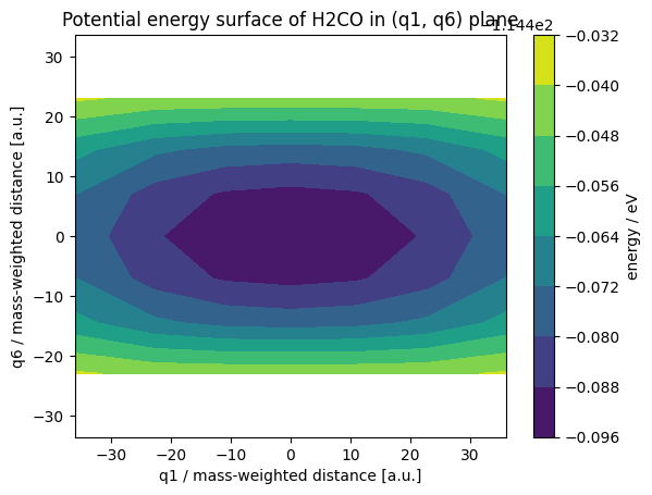
[4]:

q6, q1 = np.meshgrid(prim_info[0][5].get_grids(), prim_info[0][0].get_grids())
energy = (
    df.filter(pl.col("dofs_db") == "|0 5").sort("grids_db")["energy"].to_numpy()
)
plt.contourf(q1, q6, energy.reshape(7, 7))
plt.colorbar(label="energy / eV")
plt.xlabel("q1 / mass-weighted distance [a.u.]")
plt.ylabel("q6 / mass-weighted distance [a.u.]")
plt.title("Potential energy surface of H2CO in (q1, q6) plane")
plt.axis("equal")
plt.show()

../_images/notebook_grid-based-MPO-H2CO_11_0.png

Check MPO on :math:`J=(j_1, j_2, ldots, j_f)` index

[5]:

mpo = construct_nMR_recursive(prim_info[0], nMR=2, df=df, rate=0.99999999)
dum = None
J = [3, 3, 3, 3, 3, 3]
for j, core in zip(J, mpo, strict=False):
    if dum is None:
        dum = core[:, j, :]
    else:
        dum = np.einsum("ij,jk->ik", dum, core[:, j, :])
print(dum)  # Better to be 0.0

[[1.307280831011e-08]]

3-2 Build kinetic term

[6]:

kinetic = [[construct_kinetic_operator(dvr_prims=prim_info[0])]]

3-3 Set all operators

[7]:

ndof = len(ngrids)
potential = [[{tuple([k for k in range(ndof)]): TensorOperator(mpo=mpo)}]]
hamiltonian = TensorHamiltonian(ndof, potential, kinetic=kinetic, backend="jax")
operators = {"hamiltonian": hamiltonian}

4. Set wave function (MPS) and All Model

m_aux_max is the MPS bond dimension (maximum of auxiliary index \(\tau_p\))
init_weight_ESTATE is the initial electronic state weight. In this case, one is considering a single estate, thus this is ignored.
init_weight_VIB_GS is the initial vibrational ground state weight. 1.0 means the MPS of GS grid-pair which denotes the bottom of the potential energy surface is 1.0 and other terms are 0.0.

[8]:

model = Model(basinfo, operators)
nstate = 1
model.m_aux_max = 10
model.init_weight_VIB_GS = 1.0

5. Execute Calculation

time step width is defined by stepsize=0.1 fs

F.Y.I., See also documentation

NOTE

Runtype cannnot rebind. If you want to change runtype, you should restart kernel.

[9]:

jobname = f"h2co_7_grids_{model.m_aux_max}m"
simulator = Simulator(jobname, model, ci_type="MPS", backend="jax", verbose=4)
simulator.relax(maxstep=10, stepsize=0.1)

2024-10-26 20:21:51,163 - INFO:main.pytdscf._const_cls - 
     ____     __________   .____ ____   _____
    / _  |   /__  __/ _ \ / ___ / _  \ / ___/
   / /_) /_  __/ / / / ||/ /__ / / )_// /__
  /  ___/ / / / / / / / |.__  / |  __/ ___/
 /  /  / /_/ / / / /_/ /___/ /| \_/ / /
/__/   \__, /_/ /_____/_____/ \____/_/
      /____/

2024-10-26 20:21:51,164 - INFO:main.pytdscf._const_cls - Log file is ./h2co_7_grids_10m_relax/main.log
2024-10-26 20:21:51,164 - INFO:main.pytdscf.simulator_cls - Set integral of DVR basis
2024-10-26 20:21:51,167 - INFO:main.pytdscf.simulator_cls - Set initial wave function (DVR basis)
2024-10-26 20:21:51,167 - INFO:main.pytdscf.simulator_cls - Prepare MPS w.f.
2024-10-26 20:21:51,168 - INFO:main.pytdscf._mps_cls - Initial MPS: 0-state with weights 1.0
2024-10-26 20:21:51,168 - INFO:main.pytdscf._mps_cls - Initial MPS: 0-state 0-mode with weight [1. 0. 0. 0. 0. 0. 0.]
2024-10-26 20:21:51,168 - INFO:main.pytdscf._mps_cls - Initial MPS: 0-state 1-mode with weight [1. 0. 0. 0. 0. 0. 0.]
2024-10-26 20:21:51,168 - INFO:main.pytdscf._mps_cls - Initial MPS: 0-state 2-mode with weight [1. 0. 0. 0. 0. 0. 0.]
2024-10-26 20:21:51,169 - INFO:main.pytdscf._mps_cls - Initial MPS: 0-state 3-mode with weight [1. 0. 0. 0. 0. 0. 0.]
2024-10-26 20:21:51,169 - INFO:main.pytdscf._mps_cls - Initial MPS: 0-state 4-mode with weight [1. 0. 0. 0. 0. 0. 0.]
2024-10-26 20:21:51,169 - INFO:main.pytdscf._mps_cls - Initial MPS: 0-state 5-mode with weight [1. 0. 0. 0. 0. 0. 0.]
2024-10-26 20:21:51,437 - INFO:main.pytdscf.simulator_cls - Wave function is saved in wf_h2co_7_grids_10m_gs.pkl
2024-10-26 20:21:51,438 - INFO:main.pytdscf.simulator_cls - Start initial step    0.000 [fs]
2024-10-26 20:21:52,615 - INFO:main.pytdscf.simulator_cls - End     0 step; propagated    0.100 [fs]; AVG Krylov iteration: 19.00
2024-10-26 20:21:53,165 - INFO:main.pytdscf.simulator_cls - Saved wavefunction    0.900 [fs]
2024-10-26 20:21:53,237 - INFO:main.pytdscf.simulator_cls - End     9 step; propagated    0.900 [fs]; AVG Krylov iteration: 6.08
2024-10-26 20:21:53,238 - INFO:main.pytdscf.simulator_cls - End simulation and save wavefunction
2024-10-26 20:21:53,242 - INFO:main.pytdscf.simulator_cls - Wave function is saved in wf_h2co_7_grids_10m_gs.pkl

[9]:

(0.026051624508132566, <pytdscf.wavefunction.WFunc at 0x11cbf41a0>)

6. Check Log file

See f{jobname}_relax/main.log, which is defined by constructer of Simulator

[10]:

!tail h2co_7_grids_10m_relax/main.log

| pop 1.0000 | ene[eV]:  0.7089008 | time[fs]:    0.400 | elapsed[sec]:     1.00 | ci:  1.0  (ci_exp:  0.8|ci_rnm:  0.2|ci_etc:  0.0 d) |    0 MFLOPS (  0.0 s)
| pop 1.0000 | ene[eV]:  0.7089008 | time[fs]:    0.500 | elapsed[sec]:     1.04 | ci:  1.0  (ci_exp:  0.8|ci_rnm:  0.2|ci_etc:  0.0 d) |    0 MFLOPS (  0.0 s)
| pop 1.0000 | ene[eV]:  0.7089008 | time[fs]:    0.600 | elapsed[sec]:     1.08 | ci:  1.1  (ci_exp:  0.8|ci_rnm:  0.2|ci_etc:  0.0 d) |    0 MFLOPS (  0.0 s)
| pop 1.0000 | ene[eV]:  0.7089008 | time[fs]:    0.700 | elapsed[sec]:     1.12 | ci:  1.1  (ci_exp:  0.9|ci_rnm:  0.2|ci_etc:  0.0 d) |    0 MFLOPS (  0.0 s)
| pop 1.0000 | ene[eV]:  0.7089008 | time[fs]:    0.800 | elapsed[sec]:     1.16 | ci:  1.2  (ci_exp:  0.9|ci_rnm:  0.2|ci_etc:  0.0 d) |    0 MFLOPS (  0.0 s)
Saved wavefunction    0.900 [fs]
| pop 1.0000 | ene[eV]:  0.7089008 | time[fs]:    0.900 | elapsed[sec]:     1.19 | ci:  1.2  (ci_exp:  0.9|ci_rnm:  0.2|ci_etc:  0.0 d) |    0 MFLOPS (  0.0 s)
End     9 step; propagated    0.900 [fs]; AVG Krylov iteration: 6.08
End simulation and save wavefunction
Wave function is saved in wf_h2co_7_grids_10m_gs.pkl

/opt/homebrew/Cellar/python@3.12/3.12.2_1/Frameworks/Python.framework/Versions/3.12/lib/python3.12/pty.py:95: RuntimeWarning: os.fork() was called. os.fork() is incompatible with multithreaded code, and JAX is multithreaded, so this will likely lead to a deadlock.
  pid, fd = os.forkpty()

ZPE is found to be 0.7089008 eV!