Example 10 Time-dependent reduced density
This example takes a while. I recommend execution on HPC and select JAX as wrapper
This example is the same model as Example 11.
The differences are
Example 10 employs electronic states as a direct product state.
Therefore, two MPS are simulated.
Example 11 employs electronic states as a MPS site.
Therefore, single but longer MPS is simulated.
Example 10 construct MPO by SVD while Example 11 construct MPO analytically (use symbolic scheme).
Therefore, MPO constructed in Example 11 is free from numerical error.
Example 10 is slightly accurate but Example 11 is much computationally feasible when we simulate a couple of or dozens of electronic states.
Because direct product electronic state is accurate but suffers from exponential complexity.
Furthermore, single MPS embedded in a single Array is a suitable architecture for computation.
[1]:
!nvidia-smi
zsh:1: command not found: nvidia-smi
[2]:
import platform
import sys

import pytdscf

print(sys.version)
print(f"pytdscf version = {pytdscf.__version__}")
print(platform.platform())

import jax.extend

print(jax.extend.backend.get_backend().platform)
3.12.2 (main, Feb  6 2024, 20:19:44) [Clang 15.0.0 (clang-1500.1.0.2.5)]
pytdscf version = 1.0.3
macOS-14.4.1-arm64-arm-64bit
cpu
[3]:
import matplotlib.pyplot as plt
import numpy as np
from discvar import Exponential, HarmonicOscillator, Sine

from pytdscf import Model, Simulator, units
from pytdscf.hamiltonian_cls import TensorHamiltonian
References:
Morse potential is our original demonstration.
[4]:
backend = "jax"
Ω = 1532 / units.au_in_cm1  # Frequency of C=C stretching
K = 0.19 / units.au_in_eV
Q_ref = K / (Ω**1.5)
De = 2.285278e-1  # Dissociation energy 2.285278E-1 Eh = 600 kJ /mol
I = 1 / (
    4.84e-04 / units.au_in_eV
)  # inertial mass of C=C torsion (isomerization)
W0 = 3.56 / units.au_in_eV  # isomerization term
W1 = 1.19 / units.au_in_eV  # isomerization term
λ = 0.19 / units.au_in_eV  # Linear vibronic coupling term
E = 2.58 / units.au_in_eV - K**2 / 2 / Ω

use_bath = True

if use_bath:
    bath_ω = (
        np.array(
            [
                792.8,
                842.8,
                866.2,
                882.4,
                970.3,
                976.0,
                997.0,
                1017.1,
                1089.6,
                1189.0,
                1214.7,
                1238.1,
                1267.9,
                1317.0,
                1359.0,
                1389.0,
                1428.4,
                1434.9,
                1451.8,
                1572.8,
                1612.1,
                1629.2,
                1659.1,
            ]
        )
        / units.au_in_cm1
    )

    dimless_displace = np.array(
        [
            0.175,
            0.2,
            0.175,
            0.225,
            0.55,
            0.3,
            0.33,
            0.45,
            0.125,
            0.175,
            0.44,
            0.5,
            0.475,
            0.238,
            0.25,
            0.25,
            0.25,
            0.225,
            0.225,
            0.25,
            0.225,
            0.125,
            0.225,
        ]
    )  # c=κ/ω
[5]:
basis = [
    Sine(ngrid=2**6, length=175.0, x0=-55.0, units="a.u."),
    Exponential(ngrid=2**8 - 1, length=2 * np.pi, x0=-np.pi),
]
if use_bath:
    for ω, c in zip(bath_ω, dimless_displace, strict=False):
        ho_grids = HarmonicOscillator(10, ω, units="a.u.").get_grids()
        left_grid = ho_grids[0] - c / np.sqrt(ω)
        length = ho_grids[-1] - ho_grids[0] + c / np.sqrt(ω)  ## c=κ/ω
        basis.append(
            Sine(ngrid=2**5, length=length, x0=left_grid, units="a.u.")
        )
[6]:
s1_func = {}
s1_func[(0,)] = (
    lambda Q0: De
    * (1.0 - np.exp(-1.0 * np.sqrt(Ω**2 / 2.0 / De) * (Q0 - Q_ref))) ** 2
)
s1_func[(1,)] = lambda θ1: -W1 / 2.0 * (1.0 - np.cos(θ1))
s0_func = {}
s0_func[(0,)] = (
    lambda Q0: De * (1.0 - np.exp(-1.0 * np.sqrt(Ω**2 / 2.0 / De) * Q0)) ** 2
)
s0_func[(1,)] = lambda θ1: W0 / 2.0 * (1.0 - np.cos(θ1))
v01_func = {}
v01_func[(0,)] = lambda Q0: λ * np.sqrt(Ω) * Q0
if use_bath:
    for i in range(len(bath_ω)):
        # Be careful to late binding
        s0_func[(i + 2,)] = lambda Qi, i=i: bath_ω[i] ** 2 / 2 * Qi**2
        s1_func[(i + 2,)] = (
            lambda Qi, i=i: bath_ω[i] ** 2 / 2 * Qi**2
            + dimless_displace[i] * (bath_ω[i] ** 1.5) * Qi
        )
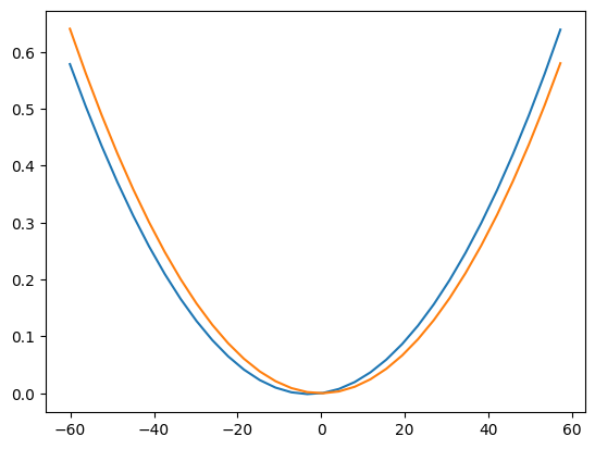
[7]:
if use_bath:
    plt.plot(
        x := np.array(basis[2].get_grids()), (s1_func[(2,)](x)) * units.au_in_eV
    )
    plt.plot(
        x := np.array(basis[2].get_grids()), s0_func[(2,)](x) * units.au_in_eV
    )
    plt.show()
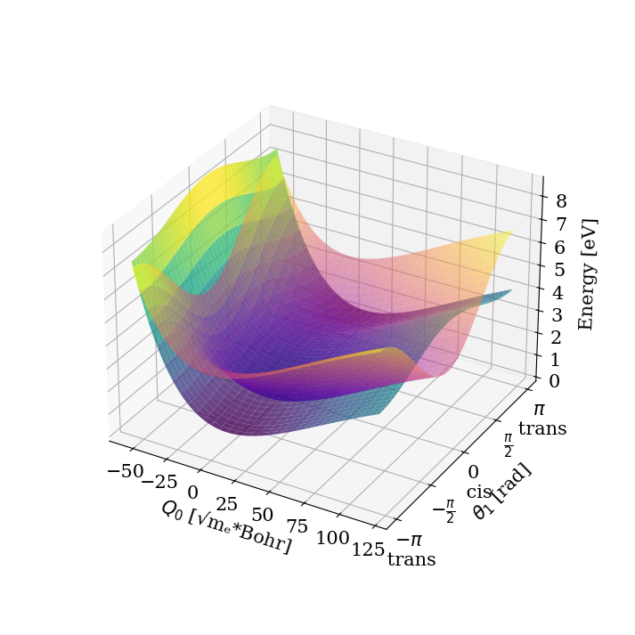
[8]:
def S1(Q, θ):
    return s1_func[(0,)](Q) + s1_func[(1,)](θ) + E


def S0(Q, θ):
    return s0_func[(0,)](Q) + s0_func[(1,)](θ)


plt.rcParams["font.size"] = 15
plt.rcParams["font.family"] = "DejaVu Serif"
Q, θ = np.meshgrid(basis[0].get_grids(), basis[1].get_grids())
V11 = (S1(Q, θ)) * units.au_in_eV
V00 = (S0(Q, θ)) * units.au_in_eV
fig = plt.figure(figsize=(9, 9))
ax = fig.add_subplot(111, projection="3d")
ax.set_xlabel("$Q_0$ [√mₑ*Bohr]")
ax.xaxis.labelpad = 10
ax.set_ylabel(r"$\theta_1$ [rad]")
ax.yaxis.labelpad = 15
ax.set_zlabel("Energy [eV]")
ax.zaxis.labelpad = 10
ax.set_yticks(
    [-np.pi, -np.pi / 2.0, 0.0, np.pi / 2.0, np.pi],
    [
        "$-\\pi$ \n trans",
        r"$-\frac{\pi}{2}$",
        "0 \n cis",
        r"$\frac{\pi}{2}$",
        "$\\pi$ \n trans",
    ],
)
surf = ax.plot_surface(Q, θ, V00, cmap="plasma", alpha=0.5)
surf = ax.plot_surface(Q, θ, V11, cmap="viridis", alpha=0.8)
ax.set_box_aspect(aspect=None, zoom=0.8)
plt.show()
[9]:
from pytdscf.dvr_operator_cls import (
    TensorOperator,
    construct_kinetic_operator,
    construct_nMR_recursive,
)

mpo_11 = construct_nMR_recursive(basis, nMR=1, func=s1_func, rate=0.99999999999)
mpo_00 = construct_nMR_recursive(basis, nMR=1, func=s0_func, rate=0.99999999999)
mpo_01 = construct_nMR_recursive(
    basis[0:1], nMR=1, func=v01_func, rate=0.99999999999
)
[10]:
# MPO has legs on (0,1,2, ... ,f-1) sites. This legs are given by tuple key
V11 = {tuple([k for k in range(len(basis))]): TensorOperator(mpo=mpo_11)}
V00 = {tuple([k for k in range(len(basis))]): TensorOperator(mpo=mpo_00)}
V01 = {(0,): TensorOperator(mpo=mpo_01, legs=(0,))}

# constant shift term is given by empty () which means no legs of tensor
# Eshift = 0.0 / units.au_in_eV
coupleJ = [[-E / 2, 0], [0, E / 2]]
V11[()] = coupleJ[1][1]
V00[()] = coupleJ[0][0]
V01[()] = coupleJ[0][1]

potential = [[V00, V01], [V01, V11]]

# Kinetic energy operator is given by
K00 = construct_kinetic_operator(
    basis, coefs=[1.0, 1.0 / I] + [1.0] * (len(basis) - 2)
)
kinetic = [[K00, None], [None, K00]]

H = TensorHamiltonian(
    ndof=len(basis), potential=potential, kinetic=kinetic, backend=backend
)

operators = {"hamiltonian": H}
[11]:
model = Model([basis, basis], operators=operators, bond_dim=20)
[12]:
def get_initial_state(ω, x):
    weight = np.exp(-ω / 2 * (np.array(x)) ** 2)
    weight /= np.linalg.norm(weight)
    return weight.tolist()


ω_list = [Ω, 2 / (0.15228**2)]
if use_bath:
    ω_list += bath_ω.tolist()
# I wonder where 0.15228 comes from???
# but https://pubs.acs.org/doi/epdf/10.1021/acs.jctc.2c00209 adopts this value
# as an initial Gaussian width of the torsional mode

init_vib = [
    get_initial_state(ω, bas.get_grids())
    for ω, bas in zip(ω_list, basis, strict=True)
]
model.init_weight_VIBSTATE = [init_vib, init_vib]
model.init_weight_ESTATE = [0.0, 1.0]
[13]:
jobname = "isomerization"
if use_bath:
    jobname += "_bath"
simulator = Simulator(jobname=jobname, model=model, backend=backend, verbose=2)
simulator.propagate(
    maxstep=4000,
    stepsize=0.05,
    reduced_density=([(0, 1)], 40),
    energy=False,
    autocorr=False,
)
# calculate (0,1) reduced density every 20 steps
2024-11-28 19:14:35,910 - INFO:main.pytdscf._const_cls -
     ____     __________   .____ ____   _____
    / _  |   /__  __/ _ \ / ___ / _  \ / ___/
   / /_) /_  __/ / / / ||/ /__ / / )_// /__
  /  ___/ / / / / / / / |.__  / |  __/ ___/
 /  /  / /_/ / / / /_/ /___/ /| \_/ / /
/__/   \__, /_/ /_____/_____/ \____/_/
      /____/

2024-11-28 19:14:35,910 - INFO:main.pytdscf._const_cls - Log file is ./isomerization_bath_prop/main.log
2024-11-28 19:14:35,910 - INFO:main.pytdscf.simulator_cls - Set integral of DVR basis
2024-11-28 19:14:35,911 - INFO:main.pytdscf.simulator_cls - Set initial wave function (DVR basis)
2024-11-28 19:14:35,912 - INFO:main.pytdscf.simulator_cls - Prepare MPS w.f.
2024-11-28 19:14:35,912 - INFO:main.pytdscf._mps_cls - Initial MPS: 0-state with weights 0.0
2024-11-28 19:14:35,912 - INFO:main.pytdscf._mps_cls - Initial MPS: 1-state with weights 1.0
2024-11-28 19:14:36,110 - INFO:main.pytdscf.simulator_cls - Wave function is saved in wf_isomerization_bath.pkl
2024-11-28 19:14:36,127 - INFO:main.pytdscf.simulator_cls - Start initial step    0.000 [fs]
2024-11-28 19:14:56,390 - INFO:main.pytdscf.simulator_cls - End     0 step; propagated    0.050 [fs]; AVG Krylov iteration: 6.82
2024-11-28 19:19:19,408 - INFO:main.pytdscf.simulator_cls - End   100 step; propagated    5.050 [fs]; AVG Krylov iteration: 6.98
2024-11-28 19:23:23,393 - INFO:main.pytdscf.simulator_cls - End   200 step; propagated   10.050 [fs]; AVG Krylov iteration: 6.63
2024-11-28 19:27:24,833 - INFO:main.pytdscf.simulator_cls - End   300 step; propagated   15.050 [fs]; AVG Krylov iteration: 6.48
2024-11-28 19:31:25,621 - INFO:main.pytdscf.simulator_cls - End   400 step; propagated   20.050 [fs]; AVG Krylov iteration: 6.41
2024-11-28 19:35:31,346 - INFO:main.pytdscf.simulator_cls - End   500 step; propagated   25.050 [fs]; AVG Krylov iteration: 6.37
2024-11-28 19:39:31,784 - INFO:main.pytdscf.simulator_cls - End   600 step; propagated   30.050 [fs]; AVG Krylov iteration: 6.34
2024-11-28 19:43:34,072 - INFO:main.pytdscf.simulator_cls - End   700 step; propagated   35.050 [fs]; AVG Krylov iteration: 6.32
2024-11-28 19:47:34,565 - INFO:main.pytdscf.simulator_cls - End   800 step; propagated   40.050 [fs]; AVG Krylov iteration: 6.30
2024-11-28 19:51:35,803 - INFO:main.pytdscf.simulator_cls - End   900 step; propagated   45.050 [fs]; AVG Krylov iteration: 6.29
2024-11-28 19:55:36,012 - INFO:main.pytdscf.simulator_cls - Saved wavefunction   49.950 [fs]
2024-11-28 19:55:41,105 - INFO:main.pytdscf.simulator_cls - End  1000 step; propagated   50.050 [fs]; AVG Krylov iteration: 6.28
2024-11-28 19:59:53,265 - INFO:main.pytdscf.simulator_cls - End  1100 step; propagated   55.050 [fs]; AVG Krylov iteration: 6.27
2024-11-28 20:04:08,619 - INFO:main.pytdscf.simulator_cls - End  1200 step; propagated   60.050 [fs]; AVG Krylov iteration: 6.26
2024-11-28 20:08:27,947 - INFO:main.pytdscf.simulator_cls - End  1300 step; propagated   65.050 [fs]; AVG Krylov iteration: 6.25
2024-11-28 20:12:56,916 - INFO:main.pytdscf.simulator_cls - End  1400 step; propagated   70.050 [fs]; AVG Krylov iteration: 6.25
2024-11-28 20:17:25,982 - INFO:main.pytdscf.simulator_cls - End  1500 step; propagated   75.050 [fs]; AVG Krylov iteration: 6.24
2024-11-28 20:21:54,178 - INFO:main.pytdscf.simulator_cls - End  1600 step; propagated   80.050 [fs]; AVG Krylov iteration: 6.24
2024-11-28 20:26:26,032 - INFO:main.pytdscf.simulator_cls - End  1700 step; propagated   85.050 [fs]; AVG Krylov iteration: 6.23
2024-11-28 20:30:57,945 - INFO:main.pytdscf.simulator_cls - End  1800 step; propagated   90.050 [fs]; AVG Krylov iteration: 6.23
2024-11-28 20:35:37,821 - INFO:main.pytdscf.simulator_cls - End  1900 step; propagated   95.050 [fs]; AVG Krylov iteration: 6.22
2024-11-28 20:40:02,979 - INFO:main.pytdscf.simulator_cls - Saved wavefunction   99.950 [fs]
2024-11-28 20:40:08,632 - INFO:main.pytdscf.simulator_cls - End  2000 step; propagated  100.050 [fs]; AVG Krylov iteration: 6.22
2024-11-28 20:44:42,813 - INFO:main.pytdscf.simulator_cls - End  2100 step; propagated  105.050 [fs]; AVG Krylov iteration: 6.21
2024-11-28 20:49:16,184 - INFO:main.pytdscf.simulator_cls - End  2200 step; propagated  110.050 [fs]; AVG Krylov iteration: 6.21
2024-11-28 20:53:50,492 - INFO:main.pytdscf.simulator_cls - End  2300 step; propagated  115.050 [fs]; AVG Krylov iteration: 6.21
2024-11-28 20:58:25,986 - INFO:main.pytdscf.simulator_cls - End  2400 step; propagated  120.050 [fs]; AVG Krylov iteration: 6.20
2024-11-28 21:02:59,426 - INFO:main.pytdscf.simulator_cls - End  2500 step; propagated  125.050 [fs]; AVG Krylov iteration: 6.20
2024-11-28 21:07:32,594 - INFO:main.pytdscf.simulator_cls - End  2600 step; propagated  130.050 [fs]; AVG Krylov iteration: 6.19
2024-11-28 21:12:03,496 - INFO:main.pytdscf.simulator_cls - End  2700 step; propagated  135.050 [fs]; AVG Krylov iteration: 6.19
2024-11-28 21:16:32,174 - INFO:main.pytdscf.simulator_cls - End  2800 step; propagated  140.050 [fs]; AVG Krylov iteration: 6.18
2024-11-28 21:20:58,257 - INFO:main.pytdscf.simulator_cls - End  2900 step; propagated  145.050 [fs]; AVG Krylov iteration: 6.18
2024-11-28 21:25:14,970 - INFO:main.pytdscf.simulator_cls - Saved wavefunction  149.950 [fs]
2024-11-28 21:25:20,321 - INFO:main.pytdscf.simulator_cls - End  3000 step; propagated  150.050 [fs]; AVG Krylov iteration: 6.17
2024-11-28 21:29:55,630 - INFO:main.pytdscf.simulator_cls - End  3100 step; propagated  155.050 [fs]; AVG Krylov iteration: 6.16
2024-11-28 21:34:42,623 - INFO:main.pytdscf.simulator_cls - End  3200 step; propagated  160.050 [fs]; AVG Krylov iteration: 6.15
2024-11-28 21:39:13,709 - INFO:main.pytdscf.simulator_cls - End  3300 step; propagated  165.050 [fs]; AVG Krylov iteration: 6.14
2024-11-28 21:44:03,088 - INFO:main.pytdscf.simulator_cls - End  3400 step; propagated  170.050 [fs]; AVG Krylov iteration: 6.12
2024-11-28 21:48:35,322 - INFO:main.pytdscf.simulator_cls - End  3500 step; propagated  175.050 [fs]; AVG Krylov iteration: 6.11
2024-11-28 21:52:46,160 - INFO:main.pytdscf.simulator_cls - End  3600 step; propagated  180.050 [fs]; AVG Krylov iteration: 6.10
2024-11-28 21:56:57,399 - INFO:main.pytdscf.simulator_cls - End  3700 step; propagated  185.050 [fs]; AVG Krylov iteration: 6.09
2024-11-28 22:01:09,593 - INFO:main.pytdscf.simulator_cls - End  3800 step; propagated  190.050 [fs]; AVG Krylov iteration: 6.07
2024-11-28 22:05:19,055 - INFO:main.pytdscf.simulator_cls - End  3900 step; propagated  195.050 [fs]; AVG Krylov iteration: 6.06
2024-11-28 22:09:28,889 - INFO:main.pytdscf.simulator_cls - Saved wavefunction  199.950 [fs]
2024-11-28 22:09:31,465 - INFO:main.pytdscf.simulator_cls - End  3999 step; propagated  199.950 [fs]; AVG Krylov iteration: 6.05
2024-11-28 22:09:31,466 - INFO:main.pytdscf.simulator_cls - End simulation and save wavefunction
2024-11-28 22:09:31,517 - INFO:main.pytdscf.simulator_cls - Wave function is saved in wf_isomerization_bath.pkl
[13]:
(None, <pytdscf.wavefunction.WFunc at 0x149a6fc80>)
[14]:
import netCDF4 as nc
from matplotlib.animation import FuncAnimation
with nc.Dataset(f"{jobname}_prop/reduced_density.nc", "r") as file:
density_data_S1 = file.variables["rho_(0, 1)_1"][:]["real"]
density_data_S0 = file.variables["rho_(0, 1)_0"][:]["real"]
time_data = file.variables["time"][:]
print(time_data.shape)
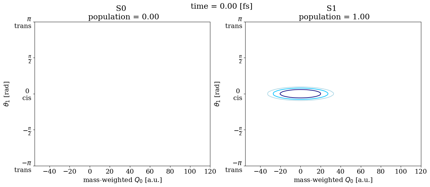
fig, (ax0, ax1) = plt.subplots(1, 2, figsize=(16, 6))
def update(i):
ax0.cla()
ax1.cla()
im0 = ax0.contour(
Q,
θ,
density_data_S0[i, :, :].T,
levels=[1.0e-05, 1.0e-04, 1.0e-03],
colors=["lightblue", "deepskyblue", "navy"],
)
# cmap='jet', vmin=0, vmax=0.05, )
im1 = ax1.contour(
Q,
θ,
density_data_S1[i, :, :].T,
levels=[1.0e-05, 1.0e-04, 1.0e-03],
colors=["lightblue", "deepskyblue", "navy"],
)
# fix coordinate of title
fig.suptitle(f"time = {time_data[i]:4.2f} [fs]")
ax0.set_title(f"S0 \n population = {np.sum(density_data_S0[i]):0.2f}")
ax1.set_title(f"S1 \n population = {np.sum(density_data_S1[i]):0.2f}")
ax0.set_xlabel("mass-weighted $Q_0$ [a.u.]")
ax1.set_xlabel("mass-weighted $Q_0$ [a.u.]")
ax0.set_ylabel(r"$\theta_1$ [rad]")
ax1.set_ylabel(r"$\theta_1$ [rad]")
ax0.set_yticks(
[-np.pi, -np.pi / 2.0, 0.0, np.pi / 2.0, np.pi],
[
"$-\\pi$ \n trans",
r"$-\frac{\pi}{2}$",
"0 \n cis",
r"$\frac{\pi}{2}$",
"$\\pi$ \n trans",
],
)
ax1.set_yticks(
[-np.pi, -np.pi / 2.0, 0.0, np.pi / 2.0, np.pi],
[
"$-\\pi$ \n trans",
r"$-\frac{\pi}{2}$",
"0 \n cis",
r"$\frac{\pi}{2}$",
"$\\pi$ \n trans",
],
)
return im0, im1
anim = FuncAnimation(fig, update, frames=range(0, len(time_data)), interval=100)
if use_bath:
gif_name = "reduced_density_bath.gif"
else:
gif_name = "reduced_density_zerotemp.gif"
anim.save(gif_name, writer="pillow")
(100,)