Example 11 Time-dependent reduced density

This example takes a while. I recommend execution on HPC and select JAX as wrapper

This example is the same model as Example 10.

The differences are

Example 10 employs electronic states as a direct product state.
- Therefore, two MPS are simulated.
Example 11 employs electronic states as a MPS site.
- Therefore, single but longer MPS is simulated.
Example 10 construct MPO by SVD while Example 11 construct MPO analytically (use symbolic scheme).
- Therefore, MPO constructed in Example 11 is free from numerical error.
Example 10 is slightly accurate but Example 11 is much computationally feasible when we simulate a couple of or dozens of electronic states.
- Because direct product electronic state is accurate but suffers from exponential complexity.
- Furthermore, single MPS embedded in a single Array is a suitable architecture for computation.

[1]:

!nvidia-smi

zsh:1: command not found: nvidia-smi

[2]:

import platform
import sys

import pytdscf

print(sys.version)
print(f"pytdscf version = {pytdscf.__version__}")
print(platform.platform())

import jax.extend

print(jax.extend.backend.get_backend().platform)

3.13.2 (main, Feb  4 2025, 14:51:09) [Clang 16.0.0 (clang-1600.0.26.6)]
pytdscf version = 1.1.0
macOS-15.4.1-arm64-arm-64bit-Mach-O
cpu

[3]:

import matplotlib.pyplot as plt
import numpy as np
import random
import sympy
from discvar import Exponential, HarmonicOscillator, Sine
from pympo import AssignManager, OpSite, SumOfProducts

from pytdscf import BasInfo, Exciton, Model, Simulator, units
from pytdscf.dvr_operator_cls import TensorOperator
from pytdscf.hamiltonian_cls import TensorHamiltonian

\[\begin{split}\begin{align} \hat{H} &= \left[-\frac{1}{2} \frac{\partial^2}{\partial Q_1^2} - \frac{1}{2I} \frac{\partial^2}{\partial \theta_2^2} - \sum_{j=3}^{25} \frac{1}{2} \frac{\partial^2}{\partial Q_{j}^2} \right] \begin{pmatrix} 1 & 0 \\ 0 & 1 \end{pmatrix} \\ &+ \begin{pmatrix} D_e\left(1-\exp\left(-\sqrt{\frac{\Omega^2}{2D_e}}Q_1\right)\right)^2 - \frac{E}{2} & \lambda Q_1 \\ \lambda Q_1 & D_e\left(1-\exp\left(-\sqrt{\frac{\Omega^2}{2D_e}}(Q_1-Q_{\mathrm{ref}})\right)\right)^2 + \frac{E}{2} \end{pmatrix} \\ &+ \begin{pmatrix} \frac{W_0}{2}\left(1-\cos\theta_2\right) & 0\\ 0 & -\frac{W_1}{2}\left(1-\cos\theta_2\right) \end{pmatrix} \\ &+\sum_{j=3}^{25} \begin{pmatrix} \frac{\omega_j^2}{2}Q_j^2 & 0 \\ 0 & \frac{\omega_j^2}{2}Q_j^2+ \kappa_j Q_j \end{pmatrix} \end{align}\end{split}\]

References:

Johnson, Philip JM, et al. “The primary photochemistry of vision occurs at the molecular speed limit.” The Journal of Physical Chemistry B 121.16 (2017): 4040-4047.
Morse potential is our original demonstration.

The second quantized representation is given by

\[\hat{T} = \left( \hat{a}_0 \hat{a}_0^\dagger + \hat{a}_0^\dagger \hat{a}_0 \right) \left( -\frac{1}{2} \frac{\partial^2}{\partial Q_1^2} -\frac{1}{2I} \frac{\partial^2}{\partial \theta_2^2} -\sum_{j=3}^{25} \frac{1}{2} \frac{\partial^2}{\partial Q_j^2} \right)\]

\[\begin{split}\begin{align*} \hat{V} &= \hat{a}_0 \hat{a}_0^\dagger \left( -\frac{E}{2} + D_e\left(1-\exp\left(-\sqrt{\frac{\Omega^2}{2D_e}}Q_1\right)\right)^2 + \frac{W_0}{2}\left(1-\cos\theta_2\right) + \sum_{j=3}^{25} \frac{\omega_j^2}{2} Q_j^2 \right)\\ &+ \hat{a}_0^\dagger \hat{a}_0 \left( \frac{E}{2} + D_e\left(1-\exp\left(-\sqrt{\frac{\Omega^2}{2D_e}}(Q_1-Q_{\mathrm{ref}})\right)\right)^2 - \frac{W_1}{2}\left(1-\cos\theta_2\right) + \sum_{j=3}^{25} \frac{\omega_j^2}{2} Q_j^2 + \kappa_j Q_j \right) \\ &+ \left(\hat{a}_0 + \hat{a}_0^\dagger\right) \lambda Q_1 \end{align*}\end{split}\]

Setup numerical parameters

[4]:

backend = "jax"
use_bath = True

Ω = 1532 / units.au_in_cm1
K = 0.19 / units.au_in_eV
De = 2.285278e-1  # Dissociation energy 2.285278E-1 Eh = 600 kJ /mol
Q_ref = K / (Ω**1.5)

I = sympy.Symbol("I")
W0 = sympy.Symbol("W_0")
W1 = sympy.Symbol("W_1")
λ = sympy.Symbol("lambda")
E = sympy.Symbol("E")


subs = {}
subs[I] = 1 / (
    4.84e-04 / units.au_in_eV
)  # inertial mass　of C=C torsion (isomerization)
subs[W0] = 3.56 / units.au_in_eV  # isomerization term
subs[W1] = 1.19 / units.au_in_eV  # isomerization term
subs[λ] = 0.19 / units.au_in_eV * np.sqrt(Ω)  # Linear vibronic coupling term
subs[E] = 2.58 / units.au_in_eV - K**2 / 2 / Ω

if use_bath:
    bath_ω = (
        np.array(
            [
                792.8,
                842.8,
                866.2,
                882.4,
                970.3,
                976.0,
                997.0,
                1017.1,
                1089.6,
                1189.0,
                1214.7,
                1238.1,
                1267.9,
                1317.0,
                1359.0,
                1389.0,
                1428.4,
                1434.9,
                1451.8,
                1572.8,
                1612.1,
                1629.2,
                1659.1,
            ]
        )
        / units.au_in_cm1
    )

    dimless_displace = np.array(
        [
            0.175,
            0.2,
            0.175,
            0.225,
            0.55,
            0.3,
            0.33,
            0.45,
            0.125,
            0.175,
            0.44,
            0.5,
            0.475,
            0.238,
            0.25,
            0.25,
            0.25,
            0.225,
            0.225,
            0.25,
            0.225,
            0.125,
            0.225,
        ]
    )  # c=κ/ω
    ω_symbols = [None, None, None]
    c_symbols = [None, None, None]
    for i, (ω, c) in enumerate(zip(bath_ω, dimless_displace, strict=True)):
        ω_symbols.append(sympy.Symbol(f"omega_{i + 3}"))
        c_symbols.append(sympy.Symbol(f"c_{i + 3}"))
        subs[ω_symbols[-1]] = ω
        subs[c_symbols[-1]] = c * (ω**1.5)

Setup basis for wavefunction

[5]:

basis = [
    Exciton(nstate=2),
    Sine(ngrid=2**6, length=175.0, x0=-55.0, units="a.u."),
    Exponential(ngrid=2**8 - 1, length=2 * np.pi, x0=-np.pi),
]
if use_bath:
    for ω, c in zip(bath_ω, dimless_displace, strict=False):
        ho_grids = HarmonicOscillator(10, ω, units="a.u.").get_grids()
        left_grid = ho_grids[0] - c / np.sqrt(ω)
        length = ho_grids[-1] - ho_grids[0] + c / np.sqrt(ω)  ## c=κ/ω
        basis.append(
            Sine(ngrid=2**5, length=length, x0=left_grid, units="a.u.")
        )
basinfo = BasInfo([basis])
ndim = len(basis)

Setup one particle operator

[6]:

q1_list = [None] + [np.array(basis_i.get_grids()) for basis_i in basis[1:]]
q2_list = [None] + [q1_int**2 for q1_int in q1_list[1:]]
p2_list = [None] + [
    basis_i.get_2nd_derivative_matrix_dvr() for basis_i in basis[1:]
]
morse_0 = De * (1.0 - np.exp(-1.0 * np.sqrt(Ω**2 / 2.0 / De) * q1_list[1])) ** 2
morse_1 = (
    De
    * (1.0 - np.exp(-1.0 * np.sqrt(Ω**2 / 2.0 / De) * (q1_list[1] - Q_ref)))
    ** 2
)
one_cos = 1.0 - np.cos(q1_list[2])
a = basis[0].get_annihilation_matrix()
adag = basis[0].get_creation_matrix()

p2_ops = [None] + [
    OpSite(f"p^2_{i}", i, value=p2_list[i]) for i in range(1, ndim)
]
q2_ops = [None] + [
    OpSite(f"q^2_{i}", i, value=q2_list[i]) for i in range(1, ndim)
]
q1_ops = [None] + [
    OpSite(f"q_{i}", i, value=q1_list[i]) for i in range(1, ndim)
]
morse_op_0 = OpSite("M^{(0)}_1", 1, value=morse_0)
morse_op_1 = OpSite("M^{(1)}_1", 1, value=morse_1)
cos_op = OpSite(r"(1-\cos \theta_{2})", 2, value=one_cos)
a_op = OpSite("a_0", 0, value=a)
adag_op = OpSite(r"a^\dagger_0", 0, value=adag)

Setup potential and kinetic operator

[7]:

pot_sop = SumOfProducts()

pot_sop += (-E / 2) * a_op * adag_op
pot_sop += a_op * adag_op * morse_op_0
pot_sop += (W0 / 2)* a_op * adag_op * cos_op
for i in range(3, ndim):
    pot_sop += (ω_symbols[i] ** 2 / 2) * a_op * adag_op * q2_ops[i]

pot_sop += (E / 2) * adag_op * a_op
pot_sop += adag_op * a_op * morse_op_1
pot_sop += (-W1 / 2) * adag_op * a_op * cos_op
for i in range(3, ndim):
    pot_sop += (ω_symbols[i] ** 2 / 2) * adag_op * a_op * q2_ops[i]
    pot_sop += (c_symbols[i]) * adag_op * a_op * q1_ops[i]

pot_sop += λ * (adag_op + a_op) * q1_ops[1]

pot_sop = pot_sop.simplify()
pot_sop.symbol

[7]:

$\displaystyle \frac{E a^{\dagger}_{0} a_{0}}{2} - \frac{E a_{0} a^{\dagger}_{0}}{2} + \frac{W_{0} a_{0} a^{\dagger}_{0} (1-\cos \theta_{2})}{2} - \frac{W_{1} a^{\dagger}_{0} a_{0} (1-\cos \theta_{2})}{2} + c_{10} a^{\dagger}_{0} a_{0} q_{10} + c_{11} a^{\dagger}_{0} a_{0} q_{11} + c_{12} a^{\dagger}_{0} a_{0} q_{12} + c_{13} a^{\dagger}_{0} a_{0} q_{13} + c_{14} a^{\dagger}_{0} a_{0} q_{14} + c_{15} a^{\dagger}_{0} a_{0} q_{15} + c_{16} a^{\dagger}_{0} a_{0} q_{16} + c_{17} a^{\dagger}_{0} a_{0} q_{17} + c_{18} a^{\dagger}_{0} a_{0} q_{18} + c_{19} a^{\dagger}_{0} a_{0} q_{19} + c_{20} a^{\dagger}_{0} a_{0} q_{20} + c_{21} a^{\dagger}_{0} a_{0} q_{21} + c_{22} a^{\dagger}_{0} a_{0} q_{22} + c_{23} a^{\dagger}_{0} a_{0} q_{23} + c_{24} a^{\dagger}_{0} a_{0} q_{24} + c_{25} a^{\dagger}_{0} a_{0} q_{25} + c_{3} a^{\dagger}_{0} a_{0} q_{3} + c_{4} a^{\dagger}_{0} a_{0} q_{4} + c_{5} a^{\dagger}_{0} a_{0} q_{5} + c_{6} a^{\dagger}_{0} a_{0} q_{6} + c_{7} a^{\dagger}_{0} a_{0} q_{7} + c_{8} a^{\dagger}_{0} a_{0} q_{8} + c_{9} a^{\dagger}_{0} a_{0} q_{9} + \lambda \left(a^{\dagger}_{0} + a_{0}\right) q_{1} + \frac{\omega_{10}^{2} \left(a^{\dagger}_{0} a_{0} + a_{0} a^{\dagger}_{0}\right) q^{2}_{10}}{2} + \frac{\omega_{11}^{2} \left(a^{\dagger}_{0} a_{0} + a_{0} a^{\dagger}_{0}\right) q^{2}_{11}}{2} + \frac{\omega_{12}^{2} \left(a^{\dagger}_{0} a_{0} + a_{0} a^{\dagger}_{0}\right) q^{2}_{12}}{2} + \frac{\omega_{13}^{2} \left(a^{\dagger}_{0} a_{0} + a_{0} a^{\dagger}_{0}\right) q^{2}_{13}}{2} + \frac{\omega_{14}^{2} \left(a^{\dagger}_{0} a_{0} + a_{0} a^{\dagger}_{0}\right) q^{2}_{14}}{2} + \frac{\omega_{15}^{2} \left(a^{\dagger}_{0} a_{0} + a_{0} a^{\dagger}_{0}\right) q^{2}_{15}}{2} + \frac{\omega_{16}^{2} \left(a^{\dagger}_{0} a_{0} + a_{0} a^{\dagger}_{0}\right) q^{2}_{16}}{2} + \frac{\omega_{17}^{2} \left(a^{\dagger}_{0} a_{0} + a_{0} a^{\dagger}_{0}\right) q^{2}_{17}}{2} + \frac{\omega_{18}^{2} \left(a^{\dagger}_{0} a_{0} + a_{0} a^{\dagger}_{0}\right) q^{2}_{18}}{2} + \frac{\omega_{19}^{2} \left(a^{\dagger}_{0} a_{0} + a_{0} a^{\dagger}_{0}\right) q^{2}_{19}}{2} + \frac{\omega_{20}^{2} \left(a^{\dagger}_{0} a_{0} + a_{0} a^{\dagger}_{0}\right) q^{2}_{20}}{2} + \frac{\omega_{21}^{2} \left(a^{\dagger}_{0} a_{0} + a_{0} a^{\dagger}_{0}\right) q^{2}_{21}}{2} + \frac{\omega_{22}^{2} \left(a^{\dagger}_{0} a_{0} + a_{0} a^{\dagger}_{0}\right) q^{2}_{22}}{2} + \frac{\omega_{23}^{2} \left(a^{\dagger}_{0} a_{0} + a_{0} a^{\dagger}_{0}\right) q^{2}_{23}}{2} + \frac{\omega_{24}^{2} \left(a^{\dagger}_{0} a_{0} + a_{0} a^{\dagger}_{0}\right) q^{2}_{24}}{2} + \frac{\omega_{25}^{2} \left(a^{\dagger}_{0} a_{0} + a_{0} a^{\dagger}_{0}\right) q^{2}_{25}}{2} + \frac{\omega_{3}^{2} \left(a^{\dagger}_{0} a_{0} + a_{0} a^{\dagger}_{0}\right) q^{2}_{3}}{2} + \frac{\omega_{4}^{2} \left(a^{\dagger}_{0} a_{0} + a_{0} a^{\dagger}_{0}\right) q^{2}_{4}}{2} + \frac{\omega_{5}^{2} \left(a^{\dagger}_{0} a_{0} + a_{0} a^{\dagger}_{0}\right) q^{2}_{5}}{2} + \frac{\omega_{6}^{2} \left(a^{\dagger}_{0} a_{0} + a_{0} a^{\dagger}_{0}\right) q^{2}_{6}}{2} + \frac{\omega_{7}^{2} \left(a^{\dagger}_{0} a_{0} + a_{0} a^{\dagger}_{0}\right) q^{2}_{7}}{2} + \frac{\omega_{8}^{2} \left(a^{\dagger}_{0} a_{0} + a_{0} a^{\dagger}_{0}\right) q^{2}_{8}}{2} + \frac{\omega_{9}^{2} \left(a^{\dagger}_{0} a_{0} + a_{0} a^{\dagger}_{0}\right) q^{2}_{9}}{2} + a^{\dagger}_{0} a_{0} M^{(1)}_1 + a_{0} a^{\dagger}_{0} M^{(0)}_1$

[8]:

kin_sop = SumOfProducts()

kin_sop += (-1 / 2) * (a_op * adag_op  + adag_op * a_op) * p2_ops[1]
kin_sop += (-1 / 2 / I) * (a_op * adag_op + adag_op * a_op) * p2_ops[2]
for i in range(3, ndim):
    kin_sop += (-1 / 2) * (a_op * adag_op + adag_op * a_op) * p2_ops[i]

kin_sop = kin_sop.simplify()
kin_sop.symbol

[8]:

$\displaystyle - 0.5 \left(a^{\dagger}_{0} a_{0} + a_{0} a^{\dagger}_{0}\right) p^{2}_{1} - 0.5 \left(a^{\dagger}_{0} a_{0} + a_{0} a^{\dagger}_{0}\right) p^{2}_{10} - 0.5 \left(a^{\dagger}_{0} a_{0} + a_{0} a^{\dagger}_{0}\right) p^{2}_{11} - 0.5 \left(a^{\dagger}_{0} a_{0} + a_{0} a^{\dagger}_{0}\right) p^{2}_{12} - 0.5 \left(a^{\dagger}_{0} a_{0} + a_{0} a^{\dagger}_{0}\right) p^{2}_{13} - 0.5 \left(a^{\dagger}_{0} a_{0} + a_{0} a^{\dagger}_{0}\right) p^{2}_{14} - 0.5 \left(a^{\dagger}_{0} a_{0} + a_{0} a^{\dagger}_{0}\right) p^{2}_{15} - 0.5 \left(a^{\dagger}_{0} a_{0} + a_{0} a^{\dagger}_{0}\right) p^{2}_{16} - 0.5 \left(a^{\dagger}_{0} a_{0} + a_{0} a^{\dagger}_{0}\right) p^{2}_{17} - 0.5 \left(a^{\dagger}_{0} a_{0} + a_{0} a^{\dagger}_{0}\right) p^{2}_{18} - 0.5 \left(a^{\dagger}_{0} a_{0} + a_{0} a^{\dagger}_{0}\right) p^{2}_{19} - 0.5 \left(a^{\dagger}_{0} a_{0} + a_{0} a^{\dagger}_{0}\right) p^{2}_{20} - 0.5 \left(a^{\dagger}_{0} a_{0} + a_{0} a^{\dagger}_{0}\right) p^{2}_{21} - 0.5 \left(a^{\dagger}_{0} a_{0} + a_{0} a^{\dagger}_{0}\right) p^{2}_{22} - 0.5 \left(a^{\dagger}_{0} a_{0} + a_{0} a^{\dagger}_{0}\right) p^{2}_{23} - 0.5 \left(a^{\dagger}_{0} a_{0} + a_{0} a^{\dagger}_{0}\right) p^{2}_{24} - 0.5 \left(a^{\dagger}_{0} a_{0} + a_{0} a^{\dagger}_{0}\right) p^{2}_{25} - 0.5 \left(a^{\dagger}_{0} a_{0} + a_{0} a^{\dagger}_{0}\right) p^{2}_{3} - 0.5 \left(a^{\dagger}_{0} a_{0} + a_{0} a^{\dagger}_{0}\right) p^{2}_{4} - 0.5 \left(a^{\dagger}_{0} a_{0} + a_{0} a^{\dagger}_{0}\right) p^{2}_{5} - 0.5 \left(a^{\dagger}_{0} a_{0} + a_{0} a^{\dagger}_{0}\right) p^{2}_{6} - 0.5 \left(a^{\dagger}_{0} a_{0} + a_{0} a^{\dagger}_{0}\right) p^{2}_{7} - 0.5 \left(a^{\dagger}_{0} a_{0} + a_{0} a^{\dagger}_{0}\right) p^{2}_{8} - 0.5 \left(a^{\dagger}_{0} a_{0} + a_{0} a^{\dagger}_{0}\right) p^{2}_{9} - \frac{0.5 \left(a^{\dagger}_{0} a_{0} + a_{0} a^{\dagger}_{0}\right) p^{2}_{2}}{I}$

Setup MPO

[9]:

am_pot = AssignManager(pot_sop)
am_pot.assign()
display(*am_pot.Wsym)
W_prod = sympy.Mul(*am_pot.Wsym)
print(*[f"W{i}" for i in range(am_pot.ndim)], "=")
display(W_prod[0].expand())
pot_mpo = am_pot.numerical_mpo(subs=subs)

$\displaystyle \left[\begin{matrix}a^{\dagger}_{0} + a_{0} & a^{\dagger}_{0} a_{0} & a^{\dagger}_{0} a_{0} + a_{0} a^{\dagger}_{0} & a_{0} a^{\dagger}_{0}\end{matrix}\right]$

$\displaystyle \left[\begin{matrix}0 & 0 & 0 & \lambda q_{1}\\1 & 0 & 0 & M^{(1)}_1\\0 & 0 & 1 & 0\\0 & 1 & 0 & M^{(0)}_1\end{matrix}\right]$

$\displaystyle \left[\begin{matrix}1 & 0 & - \frac{W_{1} (1-\cos \theta_{2})}{2}\\0 & 0 & - \frac{E}{2} + \frac{W_{0} (1-\cos \theta_{2})}{2}\\0 & 1 & 0\\0 & 0 & 1\end{matrix}\right]$

$\displaystyle \left[\begin{matrix}1 & 0 & c_{3} q_{3}\\0 & 1 & \frac{\omega_{3}^{2} q^{2}_{3}}{2}\\0 & 0 & 1\end{matrix}\right]$

$\displaystyle \left[\begin{matrix}0 & 1 & c_{4} q_{4}\\1 & 0 & \frac{\omega_{4}^{2} q^{2}_{4}}{2}\\0 & 0 & 1\end{matrix}\right]$

$\displaystyle \left[\begin{matrix}0 & 1 & \frac{\omega_{5}^{2} q^{2}_{5}}{2}\\1 & 0 & c_{5} q_{5}\\0 & 0 & 1\end{matrix}\right]$

$\displaystyle \left[\begin{matrix}1 & 0 & c_{6} q_{6}\\0 & 1 & \frac{\omega_{6}^{2} q^{2}_{6}}{2}\\0 & 0 & 1\end{matrix}\right]$

$\displaystyle \left[\begin{matrix}0 & 1 & c_{7} q_{7}\\1 & 0 & \frac{\omega_{7}^{2} q^{2}_{7}}{2}\\0 & 0 & 1\end{matrix}\right]$

$\displaystyle \left[\begin{matrix}0 & 1 & \frac{\omega_{8}^{2} q^{2}_{8}}{2}\\1 & 0 & c_{8} q_{8}\\0 & 0 & 1\end{matrix}\right]$

$\displaystyle \left[\begin{matrix}0 & 1 & c_{9} q_{9}\\1 & 0 & \frac{\omega_{9}^{2} q^{2}_{9}}{2}\\0 & 0 & 1\end{matrix}\right]$

$\displaystyle \left[\begin{matrix}0 & 1 & \frac{\omega_{10}^{2} q^{2}_{10}}{2}\\1 & 0 & c_{10} q_{10}\\0 & 0 & 1\end{matrix}\right]$

$\displaystyle \left[\begin{matrix}1 & 0 & c_{11} q_{11}\\0 & 1 & \frac{\omega_{11}^{2} q^{2}_{11}}{2}\\0 & 0 & 1\end{matrix}\right]$

$\displaystyle \left[\begin{matrix}0 & 1 & c_{12} q_{12}\\1 & 0 & \frac{\omega_{12}^{2} q^{2}_{12}}{2}\\0 & 0 & 1\end{matrix}\right]$

$\displaystyle \left[\begin{matrix}1 & 0 & \frac{\omega_{13}^{2} q^{2}_{13}}{2}\\0 & 1 & c_{13} q_{13}\\0 & 0 & 1\end{matrix}\right]$

$\displaystyle \left[\begin{matrix}1 & 0 & \frac{\omega_{14}^{2} q^{2}_{14}}{2}\\0 & 1 & c_{14} q_{14}\\0 & 0 & 1\end{matrix}\right]$

$\displaystyle \left[\begin{matrix}1 & 0 & \frac{\omega_{15}^{2} q^{2}_{15}}{2}\\0 & 1 & c_{15} q_{15}\\0 & 0 & 1\end{matrix}\right]$

$\displaystyle \left[\begin{matrix}0 & 1 & \frac{\omega_{16}^{2} q^{2}_{16}}{2}\\1 & 0 & c_{16} q_{16}\\0 & 0 & 1\end{matrix}\right]$

$\displaystyle \left[\begin{matrix}1 & 0 & c_{17} q_{17}\\0 & 1 & \frac{\omega_{17}^{2} q^{2}_{17}}{2}\\0 & 0 & 1\end{matrix}\right]$

$\displaystyle \left[\begin{matrix}0 & 1 & c_{18} q_{18}\\1 & 0 & \frac{\omega_{18}^{2} q^{2}_{18}}{2}\\0 & 0 & 1\end{matrix}\right]$

$\displaystyle \left[\begin{matrix}1 & 0 & \frac{\omega_{19}^{2} q^{2}_{19}}{2}\\0 & 1 & c_{19} q_{19}\\0 & 0 & 1\end{matrix}\right]$

$\displaystyle \left[\begin{matrix}1 & 0 & \frac{\omega_{20}^{2} q^{2}_{20}}{2}\\0 & 1 & c_{20} q_{20}\\0 & 0 & 1\end{matrix}\right]$

$\displaystyle \left[\begin{matrix}1 & 0 & \frac{\omega_{21}^{2} q^{2}_{21}}{2}\\0 & 1 & c_{21} q_{21}\\0 & 0 & 1\end{matrix}\right]$

$\displaystyle \left[\begin{matrix}1 & 0 & \frac{\omega_{22}^{2} q^{2}_{22}}{2}\\0 & 1 & c_{22} q_{22}\\0 & 0 & 1\end{matrix}\right]$

$\displaystyle \left[\begin{matrix}0 & 1 & \frac{\omega_{23}^{2} q^{2}_{23}}{2}\\1 & 0 & c_{23} q_{23}\\0 & 0 & 1\end{matrix}\right]$

$\displaystyle \left[\begin{matrix}0 & 1 & c_{24} q_{24}\\1 & 0 & \frac{\omega_{24}^{2} q^{2}_{24}}{2}\\0 & 0 & 1\end{matrix}\right]$

$\displaystyle \left[\begin{matrix}\frac{\omega_{25}^{2} q^{2}_{25}}{2}\\\frac{E}{2} + c_{25} q_{25}\\1\end{matrix}\right]$

W0 W1 W2 W3 W4 W5 W6 W7 W8 W9 W10 W11 W12 W13 W14 W15 W16 W17 W18 W19 W20 W21 W22 W23 W24 W25 =

$\displaystyle \frac{E a^{\dagger}_{0} a_{0}}{2} - \frac{E a_{0} a^{\dagger}_{0}}{2} + \frac{W_{0} a_{0} a^{\dagger}_{0} (1-\cos \theta_{2})}{2} - \frac{W_{1} a^{\dagger}_{0} a_{0} (1-\cos \theta_{2})}{2} + c_{10} a^{\dagger}_{0} a_{0} q_{10} + c_{11} a^{\dagger}_{0} a_{0} q_{11} + c_{12} a^{\dagger}_{0} a_{0} q_{12} + c_{13} a^{\dagger}_{0} a_{0} q_{13} + c_{14} a^{\dagger}_{0} a_{0} q_{14} + c_{15} a^{\dagger}_{0} a_{0} q_{15} + c_{16} a^{\dagger}_{0} a_{0} q_{16} + c_{17} a^{\dagger}_{0} a_{0} q_{17} + c_{18} a^{\dagger}_{0} a_{0} q_{18} + c_{19} a^{\dagger}_{0} a_{0} q_{19} + c_{20} a^{\dagger}_{0} a_{0} q_{20} + c_{21} a^{\dagger}_{0} a_{0} q_{21} + c_{22} a^{\dagger}_{0} a_{0} q_{22} + c_{23} a^{\dagger}_{0} a_{0} q_{23} + c_{24} a^{\dagger}_{0} a_{0} q_{24} + c_{25} a^{\dagger}_{0} a_{0} q_{25} + c_{3} a^{\dagger}_{0} a_{0} q_{3} + c_{4} a^{\dagger}_{0} a_{0} q_{4} + c_{5} a^{\dagger}_{0} a_{0} q_{5} + c_{6} a^{\dagger}_{0} a_{0} q_{6} + c_{7} a^{\dagger}_{0} a_{0} q_{7} + c_{8} a^{\dagger}_{0} a_{0} q_{8} + c_{9} a^{\dagger}_{0} a_{0} q_{9} + \lambda a^{\dagger}_{0} q_{1} + \lambda a_{0} q_{1} + \frac{\omega_{10}^{2} a^{\dagger}_{0} a_{0} q^{2}_{10}}{2} + \frac{\omega_{10}^{2} a_{0} a^{\dagger}_{0} q^{2}_{10}}{2} + \frac{\omega_{11}^{2} a^{\dagger}_{0} a_{0} q^{2}_{11}}{2} + \frac{\omega_{11}^{2} a_{0} a^{\dagger}_{0} q^{2}_{11}}{2} + \frac{\omega_{12}^{2} a^{\dagger}_{0} a_{0} q^{2}_{12}}{2} + \frac{\omega_{12}^{2} a_{0} a^{\dagger}_{0} q^{2}_{12}}{2} + \frac{\omega_{13}^{2} a^{\dagger}_{0} a_{0} q^{2}_{13}}{2} + \frac{\omega_{13}^{2} a_{0} a^{\dagger}_{0} q^{2}_{13}}{2} + \frac{\omega_{14}^{2} a^{\dagger}_{0} a_{0} q^{2}_{14}}{2} + \frac{\omega_{14}^{2} a_{0} a^{\dagger}_{0} q^{2}_{14}}{2} + \frac{\omega_{15}^{2} a^{\dagger}_{0} a_{0} q^{2}_{15}}{2} + \frac{\omega_{15}^{2} a_{0} a^{\dagger}_{0} q^{2}_{15}}{2} + \frac{\omega_{16}^{2} a^{\dagger}_{0} a_{0} q^{2}_{16}}{2} + \frac{\omega_{16}^{2} a_{0} a^{\dagger}_{0} q^{2}_{16}}{2} + \frac{\omega_{17}^{2} a^{\dagger}_{0} a_{0} q^{2}_{17}}{2} + \frac{\omega_{17}^{2} a_{0} a^{\dagger}_{0} q^{2}_{17}}{2} + \frac{\omega_{18}^{2} a^{\dagger}_{0} a_{0} q^{2}_{18}}{2} + \frac{\omega_{18}^{2} a_{0} a^{\dagger}_{0} q^{2}_{18}}{2} + \frac{\omega_{19}^{2} a^{\dagger}_{0} a_{0} q^{2}_{19}}{2} + \frac{\omega_{19}^{2} a_{0} a^{\dagger}_{0} q^{2}_{19}}{2} + \frac{\omega_{20}^{2} a^{\dagger}_{0} a_{0} q^{2}_{20}}{2} + \frac{\omega_{20}^{2} a_{0} a^{\dagger}_{0} q^{2}_{20}}{2} + \frac{\omega_{21}^{2} a^{\dagger}_{0} a_{0} q^{2}_{21}}{2} + \frac{\omega_{21}^{2} a_{0} a^{\dagger}_{0} q^{2}_{21}}{2} + \frac{\omega_{22}^{2} a^{\dagger}_{0} a_{0} q^{2}_{22}}{2} + \frac{\omega_{22}^{2} a_{0} a^{\dagger}_{0} q^{2}_{22}}{2} + \frac{\omega_{23}^{2} a^{\dagger}_{0} a_{0} q^{2}_{23}}{2} + \frac{\omega_{23}^{2} a_{0} a^{\dagger}_{0} q^{2}_{23}}{2} + \frac{\omega_{24}^{2} a^{\dagger}_{0} a_{0} q^{2}_{24}}{2} + \frac{\omega_{24}^{2} a_{0} a^{\dagger}_{0} q^{2}_{24}}{2} + \frac{\omega_{25}^{2} a^{\dagger}_{0} a_{0} q^{2}_{25}}{2} + \frac{\omega_{25}^{2} a_{0} a^{\dagger}_{0} q^{2}_{25}}{2} + \frac{\omega_{3}^{2} a^{\dagger}_{0} a_{0} q^{2}_{3}}{2} + \frac{\omega_{3}^{2} a_{0} a^{\dagger}_{0} q^{2}_{3}}{2} + \frac{\omega_{4}^{2} a^{\dagger}_{0} a_{0} q^{2}_{4}}{2} + \frac{\omega_{4}^{2} a_{0} a^{\dagger}_{0} q^{2}_{4}}{2} + \frac{\omega_{5}^{2} a^{\dagger}_{0} a_{0} q^{2}_{5}}{2} + \frac{\omega_{5}^{2} a_{0} a^{\dagger}_{0} q^{2}_{5}}{2} + \frac{\omega_{6}^{2} a^{\dagger}_{0} a_{0} q^{2}_{6}}{2} + \frac{\omega_{6}^{2} a_{0} a^{\dagger}_{0} q^{2}_{6}}{2} + \frac{\omega_{7}^{2} a^{\dagger}_{0} a_{0} q^{2}_{7}}{2} + \frac{\omega_{7}^{2} a_{0} a^{\dagger}_{0} q^{2}_{7}}{2} + \frac{\omega_{8}^{2} a^{\dagger}_{0} a_{0} q^{2}_{8}}{2} + \frac{\omega_{8}^{2} a_{0} a^{\dagger}_{0} q^{2}_{8}}{2} + \frac{\omega_{9}^{2} a^{\dagger}_{0} a_{0} q^{2}_{9}}{2} + \frac{\omega_{9}^{2} a_{0} a^{\dagger}_{0} q^{2}_{9}}{2} + a^{\dagger}_{0} a_{0} M^{(1)}_1 + a_{0} a^{\dagger}_{0} M^{(0)}_1$

[10]:

am_kin = AssignManager(kin_sop)
am_kin.assign()
display(*am_kin.Wsym)
W_prod = sympy.Mul(*am_kin.Wsym)
print(*[f"W{i}" for i in range(am_kin.ndim)], "=")
display(W_prod[0].expand())
kin_mpo = am_kin.numerical_mpo(subs=subs)

$\displaystyle \left[\begin{matrix}a^{\dagger}_{0} a_{0} + a_{0} a^{\dagger}_{0}\end{matrix}\right]$

$\displaystyle \left[\begin{matrix}1 & p^{2}_{1}\end{matrix}\right]$

$\displaystyle \left[\begin{matrix}- \frac{0.5 p^{2}_{2}}{I} & 1\\-0.5 & 0\end{matrix}\right]$

$\displaystyle \left[\begin{matrix}1 & 0\\- 0.5 p^{2}_{3} & 1\end{matrix}\right]$

$\displaystyle \left[\begin{matrix}1 & 0\\- 0.5 p^{2}_{4} & 1\end{matrix}\right]$

$\displaystyle \left[\begin{matrix}1 & 0\\- 0.5 p^{2}_{5} & 1\end{matrix}\right]$

$\displaystyle \left[\begin{matrix}1 & 0\\- 0.5 p^{2}_{6} & 1\end{matrix}\right]$

$\displaystyle \left[\begin{matrix}1 & 0\\- 0.5 p^{2}_{7} & 1\end{matrix}\right]$

$\displaystyle \left[\begin{matrix}1 & 0\\- 0.5 p^{2}_{8} & 1\end{matrix}\right]$

$\displaystyle \left[\begin{matrix}1 & 0\\- 0.5 p^{2}_{9} & 1\end{matrix}\right]$

$\displaystyle \left[\begin{matrix}1 & 0\\- 0.5 p^{2}_{10} & 1\end{matrix}\right]$

$\displaystyle \left[\begin{matrix}1 & 0\\- 0.5 p^{2}_{11} & 1\end{matrix}\right]$

$\displaystyle \left[\begin{matrix}1 & 0\\- 0.5 p^{2}_{12} & 1\end{matrix}\right]$

$\displaystyle \left[\begin{matrix}1 & 0\\- 0.5 p^{2}_{13} & 1\end{matrix}\right]$

$\displaystyle \left[\begin{matrix}1 & 0\\- 0.5 p^{2}_{14} & 1\end{matrix}\right]$

$\displaystyle \left[\begin{matrix}1 & 0\\- 0.5 p^{2}_{15} & 1\end{matrix}\right]$

$\displaystyle \left[\begin{matrix}1 & 0\\- 0.5 p^{2}_{16} & 1\end{matrix}\right]$

$\displaystyle \left[\begin{matrix}1 & 0\\- 0.5 p^{2}_{17} & 1\end{matrix}\right]$

$\displaystyle \left[\begin{matrix}1 & 0\\- 0.5 p^{2}_{18} & 1\end{matrix}\right]$

$\displaystyle \left[\begin{matrix}1 & 0\\- 0.5 p^{2}_{19} & 1\end{matrix}\right]$

$\displaystyle \left[\begin{matrix}1 & 0\\- 0.5 p^{2}_{20} & 1\end{matrix}\right]$

$\displaystyle \left[\begin{matrix}1 & 0\\- 0.5 p^{2}_{21} & 1\end{matrix}\right]$

$\displaystyle \left[\begin{matrix}1 & 0\\- 0.5 p^{2}_{22} & 1\end{matrix}\right]$

$\displaystyle \left[\begin{matrix}1 & 0\\- 0.5 p^{2}_{23} & 1\end{matrix}\right]$

$\displaystyle \left[\begin{matrix}1 & 0\\- 0.5 p^{2}_{24} & 1\end{matrix}\right]$

$\displaystyle \left[\begin{matrix}1\\- 0.5 p^{2}_{25}\end{matrix}\right]$

W0 W1 W2 W3 W4 W5 W6 W7 W8 W9 W10 W11 W12 W13 W14 W15 W16 W17 W18 W19 W20 W21 W22 W23 W24 W25 =

$\displaystyle - 0.5 a^{\dagger}_{0} a_{0} p^{2}_{1} - 0.5 a^{\dagger}_{0} a_{0} p^{2}_{10} - 0.5 a^{\dagger}_{0} a_{0} p^{2}_{11} - 0.5 a^{\dagger}_{0} a_{0} p^{2}_{12} - 0.5 a^{\dagger}_{0} a_{0} p^{2}_{13} - 0.5 a^{\dagger}_{0} a_{0} p^{2}_{14} - 0.5 a^{\dagger}_{0} a_{0} p^{2}_{15} - 0.5 a^{\dagger}_{0} a_{0} p^{2}_{16} - 0.5 a^{\dagger}_{0} a_{0} p^{2}_{17} - 0.5 a^{\dagger}_{0} a_{0} p^{2}_{18} - 0.5 a^{\dagger}_{0} a_{0} p^{2}_{19} - 0.5 a^{\dagger}_{0} a_{0} p^{2}_{20} - 0.5 a^{\dagger}_{0} a_{0} p^{2}_{21} - 0.5 a^{\dagger}_{0} a_{0} p^{2}_{22} - 0.5 a^{\dagger}_{0} a_{0} p^{2}_{23} - 0.5 a^{\dagger}_{0} a_{0} p^{2}_{24} - 0.5 a^{\dagger}_{0} a_{0} p^{2}_{25} - 0.5 a^{\dagger}_{0} a_{0} p^{2}_{3} - 0.5 a^{\dagger}_{0} a_{0} p^{2}_{4} - 0.5 a^{\dagger}_{0} a_{0} p^{2}_{5} - 0.5 a^{\dagger}_{0} a_{0} p^{2}_{6} - 0.5 a^{\dagger}_{0} a_{0} p^{2}_{7} - 0.5 a^{\dagger}_{0} a_{0} p^{2}_{8} - 0.5 a^{\dagger}_{0} a_{0} p^{2}_{9} - 0.5 a_{0} a^{\dagger}_{0} p^{2}_{1} - 0.5 a_{0} a^{\dagger}_{0} p^{2}_{10} - 0.5 a_{0} a^{\dagger}_{0} p^{2}_{11} - 0.5 a_{0} a^{\dagger}_{0} p^{2}_{12} - 0.5 a_{0} a^{\dagger}_{0} p^{2}_{13} - 0.5 a_{0} a^{\dagger}_{0} p^{2}_{14} - 0.5 a_{0} a^{\dagger}_{0} p^{2}_{15} - 0.5 a_{0} a^{\dagger}_{0} p^{2}_{16} - 0.5 a_{0} a^{\dagger}_{0} p^{2}_{17} - 0.5 a_{0} a^{\dagger}_{0} p^{2}_{18} - 0.5 a_{0} a^{\dagger}_{0} p^{2}_{19} - 0.5 a_{0} a^{\dagger}_{0} p^{2}_{20} - 0.5 a_{0} a^{\dagger}_{0} p^{2}_{21} - 0.5 a_{0} a^{\dagger}_{0} p^{2}_{22} - 0.5 a_{0} a^{\dagger}_{0} p^{2}_{23} - 0.5 a_{0} a^{\dagger}_{0} p^{2}_{24} - 0.5 a_{0} a^{\dagger}_{0} p^{2}_{25} - 0.5 a_{0} a^{\dagger}_{0} p^{2}_{3} - 0.5 a_{0} a^{\dagger}_{0} p^{2}_{4} - 0.5 a_{0} a^{\dagger}_{0} p^{2}_{5} - 0.5 a_{0} a^{\dagger}_{0} p^{2}_{6} - 0.5 a_{0} a^{\dagger}_{0} p^{2}_{7} - 0.5 a_{0} a^{\dagger}_{0} p^{2}_{8} - 0.5 a_{0} a^{\dagger}_{0} p^{2}_{9} - \frac{0.5 a^{\dagger}_{0} a_{0} p^{2}_{2}}{I} - \frac{0.5 a_{0} a^{\dagger}_{0} p^{2}_{2}}{I}$

Setup Hamiltonian

[11]:

# MPO has legs on (0,1,2, ... ,f-1) sites. This legs are given by tuple key
potential = [
    [
        {
            (((0, 0),) + tuple(i for i in range(1, ndim))): TensorOperator(
                mpo=pot_mpo
            )
        }
    ]
]  # key is ((0,0), 1, 2, ..., ndim-1)
kinetic = [
    [{tuple((i, i) for i in range(ndim)): TensorOperator(mpo=kin_mpo)}]
]  # key is ((0, 0), (1, 1), ..., (ndim-1, ndim-1))

H = TensorHamiltonian(
    ndof=len(basis), potential=potential, kinetic=kinetic, backend=backend
)

operators = {"hamiltonian": H}

Setup Model (basis, operators, initial states)

[12]:

model = Model(basinfo=basinfo, operators=operators)
model.m_aux_max = 20

[13]:

def get_initial_state(ω, x):
    weight = np.exp(-ω / 2 * (np.array(x)) ** 2)
    weight /= np.linalg.norm(weight)
    return weight.tolist()


ω_list = [Ω, 2 / (0.15228**2)]
if use_bath:
    ω_list += bath_ω.tolist()
# I wonder where 0.15228 comes from???
# but https://pubs.acs.org/doi/epdf/10.1021/acs.jctc.2c00209 adopts this value
# as an initial Gaussian width of the torsional mode

init_vib = [
    get_initial_state(ω, bas.get_grids())
    for ω, bas in zip(ω_list, basis[1:], strict=True)
]
model.init_HartreeProduct = [[[0.0, 1.0], *init_vib]]

Execution

[14]:

jobname = "isomerization_exciton"
if use_bath:
    jobname += "_bath"
simulator = Simulator(jobname=jobname, model=model, backend=backend, verbose=2)
simulator.propagate(
    maxstep=4000,
    stepsize=0.05,
    reduced_density=(
        [(0, 1, 2), (0,)],
        40,
    ),  # we want to know diagonal_element of (|0><0| |1><1| |2><2|) and (|0><0|)
    energy=False,
    autocorr=False,
)
# calculate (0,1) reduced density every 20 steps

00:35:04 | INFO | Log file is ./isomerization_exciton_bath_prop/main.log
00:35:04 | INFO | Wave function is saved in wf_isomerization_exciton_bath.pkl
00:35:04 | INFO | Start initial step    0.000 [fs]

00:35:09 | INFO | End     0 step; propagated    0.050 [fs]; AVG Krylov iteration: 6.46
00:36:49 | INFO | End   100 step; propagated    5.050 [fs]; AVG Krylov iteration: 6.00
00:38:28 | INFO | End   200 step; propagated   10.050 [fs]; AVG Krylov iteration: 5.88
00:40:05 | INFO | End   300 step; propagated   15.050 [fs]; AVG Krylov iteration: 5.85
00:41:40 | INFO | End   400 step; propagated   20.050 [fs]; AVG Krylov iteration: 5.85
00:43:16 | INFO | End   500 step; propagated   25.050 [fs]; AVG Krylov iteration: 5.85
00:44:51 | INFO | End   600 step; propagated   30.050 [fs]; AVG Krylov iteration: 5.85
00:46:28 | INFO | End   700 step; propagated   35.050 [fs]; AVG Krylov iteration: 5.85
00:48:06 | INFO | End   800 step; propagated   40.050 [fs]; AVG Krylov iteration: 5.85
00:49:48 | INFO | End   900 step; propagated   45.050 [fs]; AVG Krylov iteration: 5.85
00:51:26 | INFO | Saved wavefunction   49.950 [fs]
00:51:29 | INFO | End  1000 step; propagated   50.050 [fs]; AVG Krylov iteration: 5.85
00:53:10 | INFO | End  1100 step; propagated   55.050 [fs]; AVG Krylov iteration: 5.85
00:54:51 | INFO | End  1200 step; propagated   60.050 [fs]; AVG Krylov iteration: 5.85
00:56:34 | INFO | End  1300 step; propagated   65.050 [fs]; AVG Krylov iteration: 5.85
00:58:17 | INFO | End  1400 step; propagated   70.050 [fs]; AVG Krylov iteration: 5.85
00:59:58 | INFO | End  1500 step; propagated   75.050 [fs]; AVG Krylov iteration: 5.85
01:01:35 | INFO | End  1600 step; propagated   80.050 [fs]; AVG Krylov iteration: 5.85
01:03:10 | INFO | End  1700 step; propagated   85.050 [fs]; AVG Krylov iteration: 5.85
01:04:46 | INFO | End  1800 step; propagated   90.050 [fs]; AVG Krylov iteration: 5.85
01:06:21 | INFO | End  1900 step; propagated   95.050 [fs]; AVG Krylov iteration: 5.85
01:07:55 | INFO | Saved wavefunction   99.950 [fs]
01:07:57 | INFO | End  2000 step; propagated  100.050 [fs]; AVG Krylov iteration: 5.85
01:09:33 | INFO | End  2100 step; propagated  105.050 [fs]; AVG Krylov iteration: 5.85
01:11:10 | INFO | End  2200 step; propagated  110.050 [fs]; AVG Krylov iteration: 5.77
01:12:49 | INFO | End  2300 step; propagated  115.050 [fs]; AVG Krylov iteration: 5.69
01:14:28 | INFO | End  2400 step; propagated  120.050 [fs]; AVG Krylov iteration: 5.27
01:16:05 | INFO | End  2500 step; propagated  125.050 [fs]; AVG Krylov iteration: 5.19
01:17:41 | INFO | End  2600 step; propagated  130.050 [fs]; AVG Krylov iteration: 5.23
01:19:18 | INFO | End  2700 step; propagated  135.050 [fs]; AVG Krylov iteration: 5.19
01:20:55 | INFO | End  2800 step; propagated  140.050 [fs]; AVG Krylov iteration: 5.12
01:22:31 | INFO | End  2900 step; propagated  145.050 [fs]; AVG Krylov iteration: 5.12
01:24:06 | INFO | Saved wavefunction  149.950 [fs]
01:24:08 | INFO | End  3000 step; propagated  150.050 [fs]; AVG Krylov iteration: 5.08
01:25:45 | INFO | End  3100 step; propagated  155.050 [fs]; AVG Krylov iteration: 5.08
01:27:21 | INFO | End  3200 step; propagated  160.050 [fs]; AVG Krylov iteration: 5.08
01:28:58 | INFO | End  3300 step; propagated  165.050 [fs]; AVG Krylov iteration: 5.08
01:30:35 | INFO | End  3400 step; propagated  170.050 [fs]; AVG Krylov iteration: 5.08
01:32:10 | INFO | End  3500 step; propagated  175.050 [fs]; AVG Krylov iteration: 5.08
01:33:48 | INFO | End  3600 step; propagated  180.050 [fs]; AVG Krylov iteration: 5.08
01:35:25 | INFO | End  3700 step; propagated  185.050 [fs]; AVG Krylov iteration: 5.08
01:37:00 | INFO | End  3800 step; propagated  190.050 [fs]; AVG Krylov iteration: 5.08
01:38:34 | INFO | End  3900 step; propagated  195.050 [fs]; AVG Krylov iteration: 5.08
01:40:09 | INFO | Saved wavefunction  199.950 [fs]
01:40:10 | INFO | End  3999 step; propagated  199.950 [fs]; AVG Krylov iteration: 5.08
01:40:10 | INFO | End simulation and save wavefunction
01:40:10 | INFO | Wave function is saved in wf_isomerization_exciton_bath.pkl

[14]:

(None, <pytdscf.wavefunction.WFunc at 0x12fab1160>)

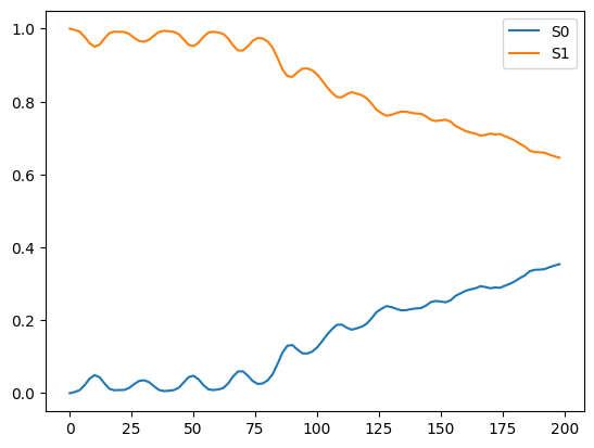
Check results (reduced densities)

[15]:

from pytdscf.util import read_nc
data = read_nc(f"{jobname}_prop/reduced_density.nc", [(0,), (0,1,2)])
time_data = data["time"]
density_data_0 = data[(0,)].real
density_data_012 = data[(0,1,2)].real

[16]:

plt.plot(time_data, density_data_0[:, 0], label="S0")
plt.plot(time_data, density_data_0[:, 1], label="S1")
plt.legend()
plt.show()

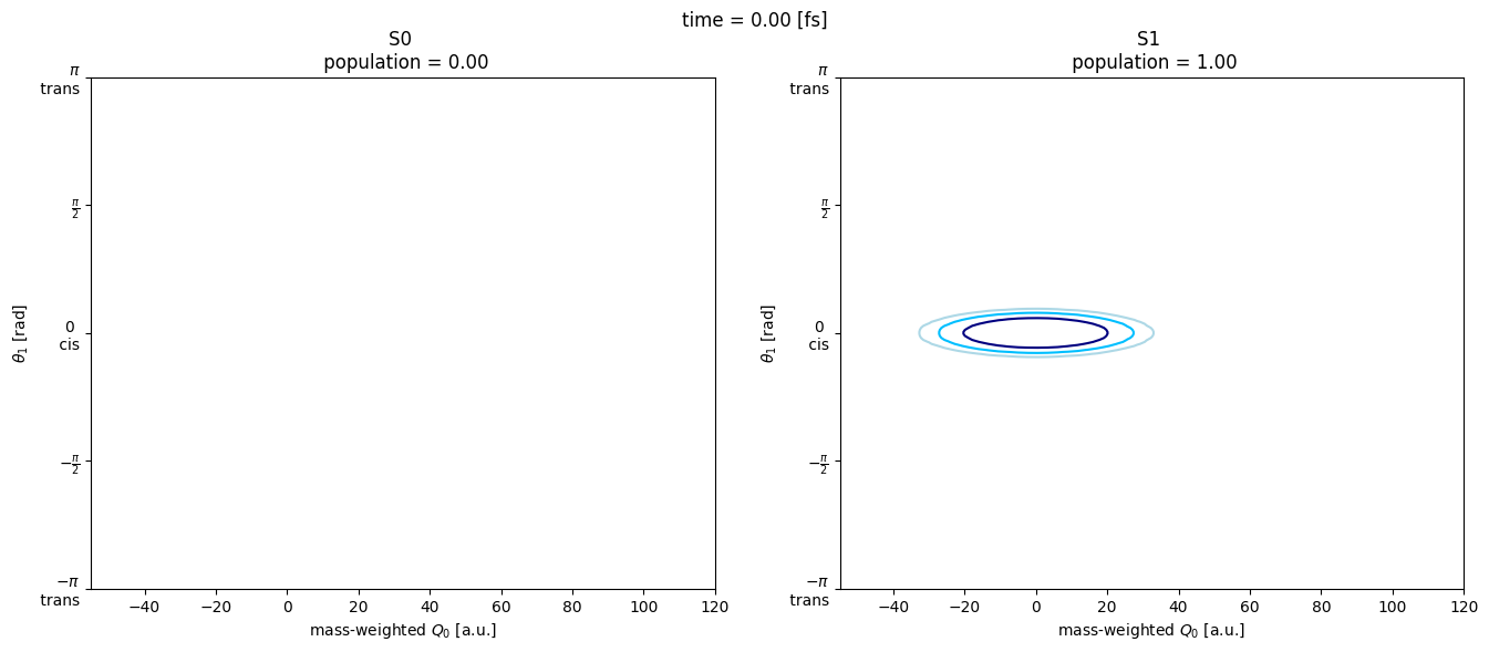
../_images/notebook_TD_reduced_density_exciton_27_0.png

[17]:

from matplotlib.animation import FuncAnimation

fig, (ax0, ax1) = plt.subplots(1, 2, figsize=(16, 6))

Q, θ = np.meshgrid(basis[1].get_grids(), basis[2].get_grids())


def update(i):
    ax0.cla()
    ax1.cla()
    im0 = ax0.contour(
        Q,
        θ,
        density_data_012[i, 0, :, :].T,
        levels=[1.0e-05, 1.0e-04, 1.0e-03],
        colors=["lightblue", "deepskyblue", "navy"],
    )
    # cmap='jet', vmin=0, vmax=0.05, )
    im1 = ax1.contour(
        Q,
        θ,
        density_data_012[i, 1, :, :].T,
        levels=[1.0e-05, 1.0e-04, 1.0e-03],
        colors=["lightblue", "deepskyblue", "navy"],
    )
    # fix coordinate of title
    fig.suptitle(f"time = {time_data[i]:4.2f} [fs]")
    ax0.set_title(
        f"S0 \n population = {np.sum(density_data_012[i, 0, :, :]):0.2f}"
    )
    ax1.set_title(
        f"S1 \n population = {np.sum(density_data_012[i, 1, :, :]):0.2f}"
    )
    ax0.set_xlabel("mass-weighted $Q_0$ [a.u.]")
    ax1.set_xlabel("mass-weighted $Q_0$ [a.u.]")
    ax0.set_ylabel(r"$\theta_1$ [rad]")
    ax1.set_ylabel(r"$\theta_1$ [rad]")
    ax0.set_yticks(
        [-np.pi, -np.pi / 2.0, 0.0, np.pi / 2.0, np.pi],
        [
            "$-\\pi$ \n trans",
            r"$-\frac{\pi}{2}$",
            "0 \n cis",
            r"$\frac{\pi}{2}$",
            "$\\pi$ \n trans",
        ],
    )
    ax1.set_yticks(
        [-np.pi, -np.pi / 2.0, 0.0, np.pi / 2.0, np.pi],
        [
            "$-\\pi$ \n trans",
            r"$-\frac{\pi}{2}$",
            "0 \n cis",
            r"$\frac{\pi}{2}$",
            "$\\pi$ \n trans",
        ],
    )
    return im0, im1


anim = FuncAnimation(fig, update, frames=range(0, len(time_data)), interval=100)
if use_bath:
    gif_name = "reduced_density_exciton_bath.gif"
else:
    gif_name = "reduced_density_exciton_zerotemp.gif"
anim.save(gif_name, writer="pillow")

../_images/notebook_TD_reduced_density_exciton_28_0.png

[ ]: