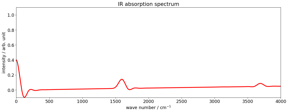
Example 4: Plot IR spectrum of H2O molecule

Documentation is here

The IR absorption spectrum is obtained by the Fourier transformation procedure

\[\begin{align} I_r(\omega) &\simeq\frac{\pi\omega}{3c\epsilon_0\hbar^2} \frac{Re}{\pi}\int_0^T e^{i(\hbar\omega+E_0)t} g(t)a_r(t) dt \end{align}\]

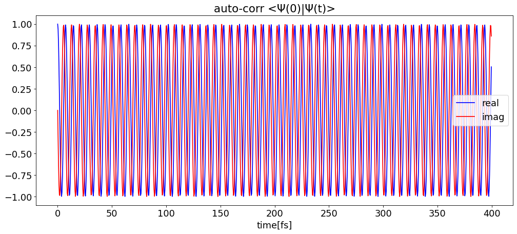
where \(a_r(t)=\langle\Psi_\mu(0)|\Psi_\mu(t)\rangle\) is an autocorrelation function, \(E_0\) can be regarded as the vibrational ground state energy and \(g(t)\) is the window function, defaults to \(g(t)=\cos^2\left(\frac{\pi t}{2T}\right)\)

1. Check autocorrelation file

[1]:

!ls h2o_polynomial_prop/autocorr*

h2o_polynomial_prop/autocorr.dat

2. Fourier transform and plot

By the so-called t/2-trick, the correlation time is twice the propagation time.

[2]:

import pytdscf

E_0 = 0.5675130  # estimated zero point energy in example 1
time, autocorr = pytdscf.spectra.load_autocorr(
    "h2o_polynomial_prop/autocorr.dat"
)
pytdscf.spectra.plot_autocorr(time, autocorr, gui=False)
freq, intensity = pytdscf.spectra.ifft_autocorr(time, autocorr, E_shift=E_0)
pytdscf.spectra.plot_spectrum(
    freq,
    intensity,
    lower_bound=0,
    upper_bound=4000,
    show_in_eV=False,
    gui=False,
)

delta_t:  0.200[fs], max_freq: 166782.0[cm-1]