Example 12 Singlet fission with bath modes
This example takes a while. (a couple of hours)
References
[1]:
import platform
import sys
import pytdscf
print(sys.version)
print(f"pytdscf version = {pytdscf.__version__}")
print(platform.platform())
import jax.extend
print(jax.extend.backend.get_backend().platform)
3.13.2 (main, Feb 4 2025, 14:51:09) [Clang 16.0.0 (clang-1600.0.26.6)]
pytdscf version = 1.1.0
macOS-15.4.1-arm64-arm-64bit-Mach-O
cpu
[2]:
import math
import matplotlib.pyplot as plt
import numpy as np
import sympy
from pympo import AssignManager, OpSite, SumOfProducts
from pympo.utils import export_npz
from pytdscf import (
Boson,
Exciton,
Model,
Simulator,
TensorHamiltonian,
TensorOperator,
units,
)
Model Hamiltonian
where \(H_{\text{ele}}\) is the electronic Hamiltonian consisting of three sites (S1, TT, CT in this order) and represented by following effective Hamiltonian
and \(H_{\text{ph}}\) and \(H_{\text{el-ph}}\) are the phonon and electron-phonon coupling Hamiltonians, respectively.
For detail derivation of this reserovir model, please refer to the reference.
We will set the electronic state as the left terminal site (i=0) and the bath modes as i=1 to N+1 sites.
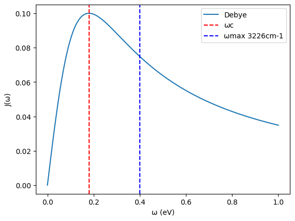
Spectral density
The previous study employed the spectral density defined as Debye type (Lorentzian decaying)
with a finite cutoff frequency \(\omega_{\text{max}}\).
[3]:
ωc = 0.18 # eV a.k.a charactaristic frequency
λ = 0.10 # eV a.k.a reorganization energy
ωmax = 0.40
def J_debye(ω):
return 2 * λ * ω * ωc / (ω * ω + ωc * ωc)
omega = np.linspace(0.0, 1.0, 1000)
plt.plot(omega, J_debye(omega), label="Debye")
plt.xlabel("ω (eV)")
plt.ylabel("J(ω)")
plt.axvline(x=ωc, color="red", linestyle="--", label="ωc")
plt.axvline(x=ωmax, color="blue", linestyle="--", label="ωmax 3226cm-1")
plt.legend()
plt.show()
The easiest transformation to finite number of harmonic oscillators is just discretizing integral
\(N\) is usually required to be a hundred number to represent the continuous spectral density.
However, there exists a more sophisticated method to map the continuous spectral density to the discrete chain with nearest neighbor coupling.
Orthogonal polynomial mapping
We will define spectral density as
where \(\theta(x)\) is the Heaviside step function. When we set \(g(x) = \omega_{\text{max}} x\) and \(x_{\text{max}}=1\), from the following relation
we can extract constant \(C=2\lambda\omega_c / \pi\) and define measure
and orthogonal monic polynomials \(\{\pi_n\}\) which satisfy
and
where \(\pi_0 = 1\) and \(\pi_{-1} = 0\).
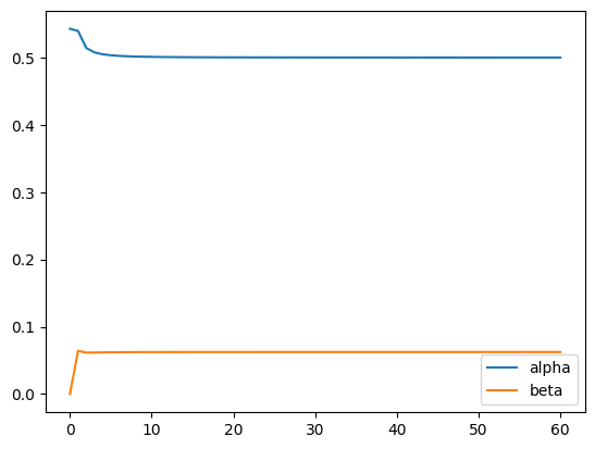
The goal is to find recursion coefficients \(\alpha_n\) and \(\beta_n\) which satisfy
and
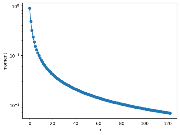
First we need to prepare the \(k\)-th moment of the measure up to \(k=2N\).
Then, we determine the coefficients \(\alpha_n\) and \(\beta_n\) recursively.
Note that recursive calculation tends to accumulate errors, so we will use mpmath to calculate the coefficients. (If you don’t have, install mpmath)
[4]:
from mpmath import mp, mpf
mp.dps = 512
def get_momments(n_order, L: float):
moments = [
mpf(1) / mpf(2) * mp.log1p(mpf(L) ** 2),
1 - mp.atan(mpf(L)) / mpf(L),
]
for k in range(2, 2 * n_order + 1):
moments.append(1 / mpf(k) - moments[-2] / mpf(L) / mpf(L))
return moments
n_order = 61
L = ωmax / ωc
moments = get_momments(n_order, L)
plt.plot(moments, marker="o")
plt.xlabel("n")
plt.ylabel("moment")
plt.yscale("log")
plt.axhline(0.0, color="black", linestyle="--")
plt.show()
[5]:
def polynomial_inner_product(
poly1: np.ndarray, poly2: np.ndarray, moments: np.ndarray
):
"""
Calculate the inner product of two polynomials using the moments.
Args:
poly1: Coefficients of the first polynomial. [1.0, 2.0, 3.0] means 1 + 2x + 3x^2
poly2: Coefficients of the second polynomial. [1.0, 2.0, 3.0] means 1 + 2x + 3x^2
moments: Moments used to calculate the inner product.
"""
assert len(poly1) + len(poly2) - 1 <= len(moments)
# convolution = np.convolve(poly1, poly2)
# return np.dot(convolution, moments[:len(convolution)])
convolution = [mpf(0)] * (len(poly1) + len(poly2) - 1)
for i in range(len(poly1)):
for j in range(len(poly2)):
convolution[i + j] += poly1[i] * poly2[j]
return sum(
c * m
for c, m in zip(convolution, moments[: len(convolution)], strict=False)
)
[6]:
def get_coef_alpha_beta_recursive(n_order, moments):
# monic_coefs = [[1.0]]
monic_coefs = [[mpf(1)]]
alpha = []
beta = []
norm = [] # <pi_k,pi_k>
for n in range(n_order):
# coefs_pi_k = [0.0] + monic_coefs[-1]
coefs_pi_k = [mpf(0)] + monic_coefs[-1]
# coefs_x_pi_k = monic_coefs[-1] + [0.0]
coefs_x_pi_k = monic_coefs[-1] + [mpf(0)]
assert coefs_x_pi_k[0] == 1.0
# <pi_k,pi_k>
alpha_denom = polynomial_inner_product(
np.array(coefs_pi_k)[::-1],
np.array(coefs_pi_k)[::-1],
np.array(moments),
)
# <x pi_k,pi_k>
alpha_num = polynomial_inner_product(
np.array(coefs_x_pi_k)[::-1],
np.array(coefs_pi_k)[::-1],
np.array(moments),
)
alpha.append(alpha_num / alpha_denom)
norm.append(alpha_denom)
if n >= 1:
beta_num = norm[-1]
beta_denom = norm[-2]
beta.append(beta_num / beta_denom)
else:
# beta.append(0.0)
beta.append(mpf(0))
monic_coefs.append(coefs_x_pi_k)
for i in range(len(monic_coefs[-2])):
monic_coefs[-1][-i - 1] -= alpha[-1] * monic_coefs[-2][-i - 1]
if n >= 1:
for i in range(len(monic_coefs[-3])):
monic_coefs[-1][-i - 1] -= beta[-1] * monic_coefs[-3][-i - 1]
return monic_coefs, alpha, beta, norm
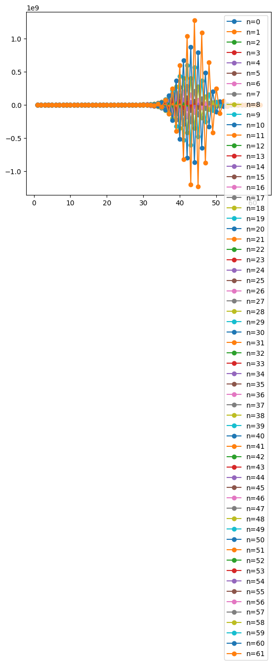
monic_coefs, alpha, beta, norm = get_coef_alpha_beta_recursive(n_order, moments)
for i in range(len(monic_coefs)):
plt.plot(
np.arange(i + 1, 0, -1), monic_coefs[i], label=f"n={i}", marker="o"
)
plt.legend()
plt.show()
plt.plot(alpha, label="alpha")
plt.plot(beta, label="beta")
plt.legend()
plt.show()
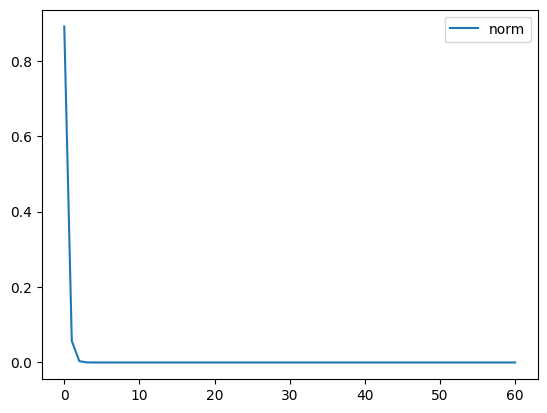
plt.plot(norm, label="norm")
plt.legend()
plt.show()
[7]:
plt.plot(np.abs(np.array(alpha) - 1 / 2) * L, label="L|alpha-1/2|", marker="o")
plt.plot(
np.abs(1 / 16 - np.array(beta)) * L * L, label="L^2|1/16-beta|", marker="x"
)
plt.yscale("log")
plt.legend()
plt.show()
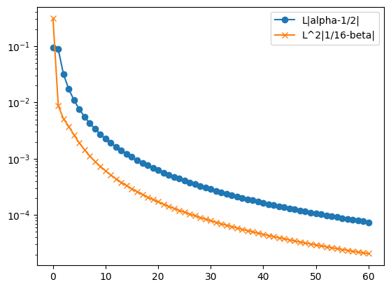
Then, we have the parameters
And total Hamiltonian is
where \(\hat{A}\) is the operator like \(\sum_{k} |k\rangle \langle k|\) acting on the electronic state.
[8]:
backend = "numpy" # "jax"
c0 = math.sqrt(λ * ωc * math.log(1 + L**2) / math.pi) / units.au_in_eV
omega = np.array(alpha, dtype=np.float64) * ωmax / units.au_in_eV
t = np.sqrt(np.array(beta[1:], dtype=np.float64)) * ωmax / units.au_in_eV
c0_sym = sympy.Symbol("c_0")
omega_syms = [sympy.Symbol(f"omega_{i}") for i in range(len(omega))]
t_syms = [sympy.Symbol(f"t_{i}") for i in range(len(t))]
subs = {}
subs[c0_sym] = c0
for omega_val, omega_sym in zip(omega, omega_syms, strict=True):
subs[omega_sym] = omega_val
for t_val, t_sym in zip(t, t_syms, strict=True):
subs[t_sym] = t_val
Setup basis for wavefunction
[9]:
basis = (
[Boson(8)] * n_order
+ [Exciton(nstate=3, names=["S1", "TT", "CS"])]
+ [Boson(8)] * (2 * n_order)
)
ndim = len(basis)
print(ndim)
sys_site = n_order
184
Setup one particle operator

[10]:
eham = (
np.array([[0.2, 0.0, -0.05], [0.0, 0.0, -0.05], [-0.05, -0.05, 0.3]])
/ units.au_in_eV
)
b = basis[0].get_annihilation_matrix()
bdag = basis[0].get_creation_matrix()
num = basis[0].get_number_matrix()
bdagb = num
s1 = np.zeros((3, 3))
s1[0, 0] = 1.0 # act only on S1
tt = np.zeros((3, 3))
tt[1, 1] = 1.0 # act only on TT
ct = np.zeros((3, 3))
ct[2, 2] = 1.0 # act only on CT
eham_op = OpSite("H_{" + f"{sys_site}" + "}", sys_site, value=eham)
s1_op = OpSite("S1" + "_{" + f"{sys_site}" + "}", sys_site, value=s1)
tt_op = OpSite(r"\text{TT}" + "_{" + f"{sys_site}" + "}", sys_site, value=tt)
ct_op = OpSite(r"\text{CT}" + "_{" + f"{sys_site}" + "}", sys_site, value=ct)
b_ops = [
OpSite("b_{" + f"{n}" + "}", n, value=b) if n != sys_site else None
for n in range(3 * n_order + 1)
]
bdag_ops = [
OpSite(r"b^\dagger" + "_{" + f"{n}" + "}", n, value=bdag)
if n != sys_site
else None
for n in range(3 * n_order + 1)
]
bdagb_ops = [
OpSite(
r"b^\dagger" + "_{" + f"{n}" + "}" + "b_{" + f"{n}" + "}",
n,
value=bdagb,
)
if n != sys_site
else None
for n in range(3 * n_order + 1)
]
Setup potential and kinetic operator
[11]:
sop = SumOfProducts()
sop += eham_op
sop += c0_sym * s1_op * (b_ops[sys_site - 1] + bdag_ops[sys_site - 1])
for i, n in enumerate(range(sys_site - 1, -1, -1)):
sop += omega_syms[i] * bdagb_ops[n]
if i != n_order - 1:
sop += t_syms[i] * (
b_ops[n] * bdag_ops[n - 1] + bdag_ops[n] * b_ops[n - 1]
)
sop += c0_sym * ct_op * (b_ops[sys_site + 1] + bdag_ops[sys_site + 1])
for i, n in enumerate(range(sys_site + 1, 3 * n_order, 2)):
sop += omega_syms[i] * bdagb_ops[n]
if i != n_order - 1:
sop += t_syms[i] * (
b_ops[n] * bdag_ops[n + 1] + bdag_ops[n] * b_ops[n + 1]
)
sop += c0_sym * tt_op * (b_ops[sys_site + 2] + bdag_ops[sys_site + 2])
for i, n in enumerate(range(sys_site + 2, 3 * n_order + 1, 2)):
sop += omega_syms[i] * bdagb_ops[n]
if i != n_order - 1:
sop += t_syms[i] * (
b_ops[n] * bdag_ops[n + 1] + bdag_ops[n] * b_ops[n + 1]
)
sop = sop.simplify()
sop.symbol
[11]:
Setup MPO
[12]:
am_pot = AssignManager(sop)
am_pot.assign()
W_prod = sympy.Mul(*am_pot.Wsym)
assert W_prod[0] == sop.symbol, W_prod[0] - sop.symbol
pot_mpo = am_pot.numerical_mpo(subs=subs)
export_npz(pot_mpo, "singlet_fission_mpo.npz")
# display(*am_pot.Wsym)
Setup Hamiltonian
[13]:
# MPO has legs on (0,1,2, ... ,f-1) sites. This legs are given by tuple key
potential = [
[{tuple((k, k) for k in range(ndim)): TensorOperator(mpo=pot_mpo)}]
] # key is ((0,0), 1, 2, ..., ndim-1)
H = TensorHamiltonian(
ndof=len(basis), potential=potential, kinetic=None, backend=backend
)
core = np.zeros((1, 3, 1))
core[0, 0, 0] = 1.0
s1 = TensorHamiltonian(
ndof=len(basis),
potential=[[{(sys_site,): TensorOperator(mpo=[core], legs=(sys_site,))}]],
kinetic=None,
backend=backend,
)
operators = {"hamiltonian": H, "S1": s1}
from itertools import chain
sites = chain(
range(sys_site - 1, -1, -4),
range(sys_site + 1, 3 * n_order + 1, 8),
range(sys_site + 2, 3 * n_order + 1, 8),
)
for isite in sites:
core = np.zeros((1, basis[isite].nprim, 1))
core[0, :, 0] = np.arange(basis[isite].nprim)
n = TensorHamiltonian(
ndof=len(basis),
potential=[[{(isite,): TensorOperator(mpo=[core], legs=(isite,))}]],
kinetic=None,
backend=backend,
)
operators[f"N{isite}"] = n
Setup Model (basis, operators, initial states)
[14]:
model = Model(basis, operators=operators, bond_dim=20)
# Starts from S1 state
init_boson = [[1.0] + [0.0] * (basis[1].nprim - 1)]
model.init_HartreeProduct = [
init_boson * n_order + [[1.0, 0.0, 0.0]] + init_boson * (2 * n_order)
]
Execution
[15]:
jobname = "singlet_fission"
simulator = Simulator(jobname=jobname, model=model, backend=backend, verbose=2)
simulator.propagate(
maxstep=2000,
stepsize=0.2,
reduced_density=(
[(sys_site, sys_site)],
10,
), # we want to know diagonal_element of (|S1><S1| |CT><CT| |TT><TT| |S1><CT| |S1><TT| |CS><TT|)
energy=False,
autocorr=False,
observables=True,
observables_per_step=10,
)
18:30:09 | INFO | Log file is ./singlet_fission_prop/main.log
18:30:09 | INFO | Wave function is saved in wf_singlet_fission.pkl
18:30:09 | INFO | Start initial step 0.000 [fs]
18:30:11 | INFO | End 0 step; propagated 0.200 [fs]; AVG Krylov iteration: 5.64
18:32:28 | INFO | End 100 step; propagated 20.200 [fs]; AVG Krylov iteration: 5.88
18:34:43 | INFO | End 200 step; propagated 40.200 [fs]; AVG Krylov iteration: 5.53
18:36:58 | INFO | End 300 step; propagated 60.200 [fs]; AVG Krylov iteration: 5.62
18:39:07 | INFO | End 400 step; propagated 80.200 [fs]; AVG Krylov iteration: 5.41
18:41:08 | INFO | End 500 step; propagated 100.200 [fs]; AVG Krylov iteration: 5.10
18:43:09 | INFO | End 600 step; propagated 120.200 [fs]; AVG Krylov iteration: 5.07
18:45:08 | INFO | End 700 step; propagated 140.200 [fs]; AVG Krylov iteration: 5.22
18:47:08 | INFO | End 800 step; propagated 160.200 [fs]; AVG Krylov iteration: 5.29
18:49:07 | INFO | End 900 step; propagated 180.200 [fs]; AVG Krylov iteration: 5.24
18:51:05 | INFO | Saved wavefunction 199.800 [fs]
18:51:08 | INFO | End 1000 step; propagated 200.200 [fs]; AVG Krylov iteration: 5.23
18:53:09 | INFO | End 1100 step; propagated 220.200 [fs]; AVG Krylov iteration: 5.19
18:55:10 | INFO | End 1200 step; propagated 240.200 [fs]; AVG Krylov iteration: 5.14
18:57:10 | INFO | End 1300 step; propagated 260.200 [fs]; AVG Krylov iteration: 5.17
18:59:11 | INFO | End 1400 step; propagated 280.200 [fs]; AVG Krylov iteration: 5.17
19:01:10 | INFO | End 1500 step; propagated 300.200 [fs]; AVG Krylov iteration: 5.12
19:03:08 | INFO | End 1600 step; propagated 320.200 [fs]; AVG Krylov iteration: 5.10
19:05:11 | INFO | End 1700 step; propagated 340.200 [fs]; AVG Krylov iteration: 5.06
19:07:08 | INFO | End 1800 step; propagated 360.200 [fs]; AVG Krylov iteration: 5.03
19:09:05 | INFO | End 1900 step; propagated 380.200 [fs]; AVG Krylov iteration: 5.02
19:10:58 | INFO | Saved wavefunction 399.800 [fs]
19:11:00 | INFO | End 1999 step; propagated 399.800 [fs]; AVG Krylov iteration: 5.01
19:11:00 | INFO | End simulation and save wavefunction
19:11:00 | INFO | Wave function is saved in wf_singlet_fission.pkl
[15]:
(None, <pytdscf.wavefunction.WFunc at 0x131f67230>)
Check results (reduced densities)
[16]:
import netCDF4 as nc
with nc.Dataset(f"{jobname}_prop/reduced_density.nc", "r") as file:
density_data_real = file.variables[f"rho_({sys_site}, {sys_site})_0"][:][
"real"
]
density_data_imag = file.variables[f"rho_({sys_site}, {sys_site})_0"][:][
"imag"
]
time_data = file.variables["time"][:]
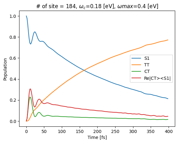
[17]:
plt.title(f"# of site = {len(basis)}, $ω_c$={ωc} [eV], $ωmax$={ωmax} [eV]")
plt.ylabel("Population")
plt.xlabel("Time [fs]")
plt.plot(time_data, density_data_real[:, 0, 0], label="S1")
plt.plot(time_data, density_data_real[:, 1, 1], label="TT")
plt.plot(time_data, density_data_real[:, 2, 2], label="CT")
plt.plot(time_data, density_data_real[:, 0, 2], label="Re|CT><S1|")
plt.legend()
plt.show()
[18]:
density_data = np.array(density_data_real) + 1.0j * np.array(density_data_imag)
time_data = np.array(time_data)
from IPython.display import HTML
from pytdscf.util.anim_density_matrix import get_anim
fig, anim = get_anim(
density_data,
time_data,
title="Reduced density matrix",
time_unit="fs",
row_names=[r"$|S1\rangle$", r"$|TT\rangle$", r"$|CT\rangle$"],
col_names=[r"$\langle S1|$", r"$\langle TT|$", r"$\langle CT|$"],
)
HTML(anim.to_jshtml())
[18]: